MATLAB与电子表格数值分析实战

下载需积分: 5 | PDF格式 | 4.64MB | 更新于2025-01-04 | 98 浏览量 | 举报

"《Numerical Analysis Using MATLAB and Spreadsheets, 2nd ed.》是Steven T. Karris撰写的一本书，旨在通过MATLAB编程语言和电子表格工具进行数值分析的实践教学。这本书的第二版提供了对数值计算的深入理解和应用。" 在书中，作者首先介绍了MATLAB的基本使用，包括： 1. 命令窗口：这是用户与MATLAB交互的主要界面，用于输入命令和查看结果。 2. 多项式根的求解：阐述如何找到多项式的根，并讨论如何从已知根构建多项式。 3. 多项式评估：教授如何在指定点上计算多项式的值。 4. 有理多项式：讲解了有理多项式的处理方法。 5. 图形绘制：利用MATLAB创建各种图形，如子图的使用，以及乘法、除法和指数运算的实现。 6. 脚本和函数文件：介绍MATLAB中的脚本文件和函数文件，用于组织和复用代码。 7. 显示格式：调整MATLAB中的显示样式和精度。接下来，书中的章节关注于根的近似计算： 1. 牛顿法：详细解释了使用牛顿迭代法寻找函数零点的过程。 2. 使用电子表格进行近似计算：展示了如何在电子表格软件中执行根的近似计算。 3. 二分法：介绍了通过不断分割区间来找寻根的二分法算法。在后续章节，书本涉及了信号处理和电路分析的主题： 1. 正弦波和相量：讨论了交流电压和电流的特性，以及正弦波的性质。 2. 反三角函数：对反三角函数进行了深入探讨，它们在工程和科学计算中扮演着重要角色。 3. 相量：引入了相量的概念，用于表示和处理复数信号，特别是在电气工程中。 4. 相量的加减和乘法：详细阐述了如何操作和组合相量，包括它们之间的加、减和乘运算。这本书是学习数值分析和利用MATLAB及电子表格工具进行实际计算的宝贵资源，涵盖了从基础到高级的多个主题，并通过练习和解答来巩固读者的理解。无论是学生还是专业人员，都能从中受益匪浅，提升在数值计算方面的技能。

Numerical Analysis Using MATLAB and Spreadsheets, Second Edition 1-9

Orchard Publications

Using MATLAB to Make Plots

1.6 Using MATLAB to Make Plots

Quite often, we want to plot a set of ordered pairs. This is a very easy task with the MATLAB

plot(x,y) command which plots versus . Here, is the horizontal axis (abscissa) and is the

vertical axis (ordinate).

Example 1.10

Consider the electric circuit of Figure 1.1, where the radian frequency (radians/second) of the

applied voltage was varied from to

in steps of radians/second, while the amplitude

was held constant. The ammeter readings were then recorded for each frequency. The magnitude

of the impedance was computed as and the data were tabulated in Table 1.1.

Figure 1.1. Electric circuit for Example 1.10

Plot the magnitude of the impedance, that is, versus radian frequency .

TABLE 1.1 Table for Example 1.10

(rads/s) Ohms (rads/s) Ohms

300 39.339 1700 90.603

400 52.589 1800 81.088

500 71.184 1900 73.588

600 97.665 2000 67.513

700 140.437 2100 62.481

800 222.182 2200 58.240

900 436.056 2300 54.611

1000 1014.938 2400 51.428

1100 469.83 2500 48.717

1200 266.032 2600 46.286

1300 187.052 2700 44.122

1400 145.751 2800 42.182

1500 120.353 2900 40.432

1600 103.111 3000 38.845

yxx y

300 3000 100

ZVA⁄=

ω Z

Z ω

Numerical Analysis Using MATLAB and Spreadsheets, Second Edition 1-11

Orchard Publications

Using MATLAB to Make Plots

To return to the command window, we press any key, or from the Window pull-down menu, we

select MATLAB Command Window. To see the graph again, we click on the Window pull-down

menu, and we select Figure.

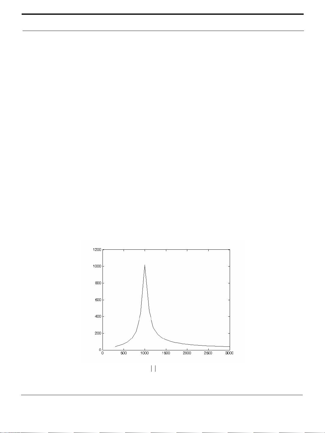
We can make the above, or any plot, more presentable with the following commands:

grid on: This command adds grid lines to the plot. The grid off command removes the grid. The

command

grid toggles them, that is, changes from off to on or vice versa. The default

is off.

box off: This command removes the box (the solid lines which enclose the plot), and box on

restores the box. The command box toggles them. The default is on.

title(‘string’): This command adds a line of the text string (label) at the top of the plot.

xlabel(‘string’) and ylabel(‘string’) are used to label the - and -axis respectively.

The amplitude frequency response is usually represented with the -axis in a logarithmic scale.

We can use the

semilogx(x,y) command that is similar to the plot(x,y) command, except that

the -axis is represented as a log scale, and the -axis as a linear scale. Likewise, the semil-

ogy(x,y)

command is similar to the plot(x,y) command, except that the -axis is represented as a

log scale, and the -axis as a linear scale. The loglog(x,y) command uses logarithmic scales for

both axes.

Throughout this text, it will be understood that log is the common (base 10) logarithm, and ln is

the natural (base e) logarithm. We must remember, however, the function log(x) in MATLAB is

the natural logarithm, whereas the common logarithm is expressed as

log10(x). Likewise, the log-

arithm to the base 2 is expressed as

log2(x).

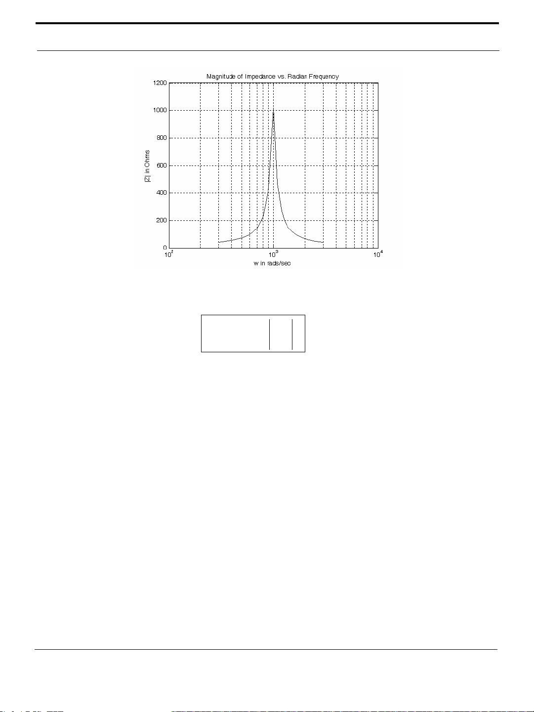
Let us now redraw the plot with the above options, by adding the following statements:

semilogx(w,z); grid; % Replaces the plot(w,z) command

title('Magnitude of Impedance vs. Radian Frequency');

xlabel('w in rads/sec'); ylabel('|Z| in Ohms')

After execution of these commands, our plot is as shown in Figure 1.3.

If the -axis represents power, voltage, or current, the -axis of the frequency response is more

often shown in a logarithmic scale, and the -axis in dB (decibels) scale. A review of the decibel

unit follows.

The ratio of any two values of the same quantity (power, voltage, or current) can be expressed in

decibels (dB). Thus, we say that an amplifier has power gain, or a transmission line has a

power loss of (or gain ). If the gain (or loss) is the output is equal to the input.

* Default is a particular value for a variable or condition that is assigned automatically by an operating system, and remains

in effect unless canceled or overridden by the operator.

10 dB

7 dB 7– dB 0 dB

剩余569页未读，继续阅读

minghuai

粉丝: 0

MATLAB与电子表格数值分析实战

"Matlab数值分析进阶教程：插值与逼近

"深入浅出MATLAB应用基础教程，适合初学者

"基于MATLAB的通信系统设计与仿真

Numerical Analysis Using MATLAB and Spreadsheets 2ed

Steven T. Karris - Numerical Analysis using Matlab and Spreadsheets, 2nd Ed

NUMERICAL ANALYSIS USING MATLAB AND EXCEL 3RD ED

Numerical Analysis Using MATLAB and Excel, 3rd Ed

Numerical Analysis Using MATLAB and Excel

Numerical Analysis Using MATLAB and Excel 第三版

Numerical Analysis for Statisticians 2nd Edition.pdf

最新资源