2015年IEEE Transactions on Image Processing论文：视觉显著对象检测基准研究

需积分: 9 166 浏览量更新于2024-07-15 收藏 12.69MB PDF 举报

本文《显著对象检测：一个基准》发表在2015年1月的IEEE Transactions on Image Processing上，由阿里·博里、明ming-明成、华如柱和佳利四位作者合作完成。该研究是视觉注意力领域的一个重要里程碑，旨在通过评估和比较40个最先进的显著对象检测算法，为计算机视觉任务提供可靠的关键区域检测方法，这些任务包括图像分割、物体识别和自适应压缩。文章的核心关注点在于提出一种基于区域对比度的显著对象检测基准，这是一种旨在衡量算法在识别图像中最具视觉吸引力或突出部分（salient objects）的能力。作者们对这些算法进行了详尽的定量和定性分析，以便确定它们在处理复杂场景和不同视觉特性（如大小、形状、纹理等）时的表现。研究中的关键贡献包括： 1. **方法评估**：通过对大量实验数据的分析，论文提供了对于各算法在处理各类场景（如自然场景、人造场景、静止图像和视频序列）下的性能评估指标，比如平均精度（mean average precision, mAP）、F-measure和AUC值等。 2. **基准设计**：设计了一个全面的评估框架，包括标准测试集和评估流程，使得研究人员可以方便地比较他们的算法与已有的方法，并推动领域内的技术进步。 3. **挑战与讨论**：文章还探讨了当前显著对象检测领域的挑战，例如光照变化、遮挡和复杂背景的影响，以及如何提高算法鲁棒性和效率。 4. **作者背景**：阿里·博里、明ming-明成来自学术界的重要机构，他们在图像增强和相关项目上也有所贡献，显示了他们在这个领域的深厚研究背景和影响力。 5. **后续影响**：这篇论文被引用次数超过600次，表明其在显著对象检测领域的广泛认可和研究价值，同时也促进了其他相关项目的进展，如ImageEnhancement。《SalientObjectDetection: A Benchmark》是一篇深入研究和比较显著对象检测技术的重要论文，为后续研究者提供了一个清晰的评估标准，有助于推动计算机视觉领域的发展。如果你需要进行显著对象检测相关的项目或者研究，这篇文章将为你提供宝贵的参考资源和比较依据。

IEEE TRANSACTIONS ON IMAGE PROCESSING, VOL. XXX, NO. XXX, XXXXX 2014 3

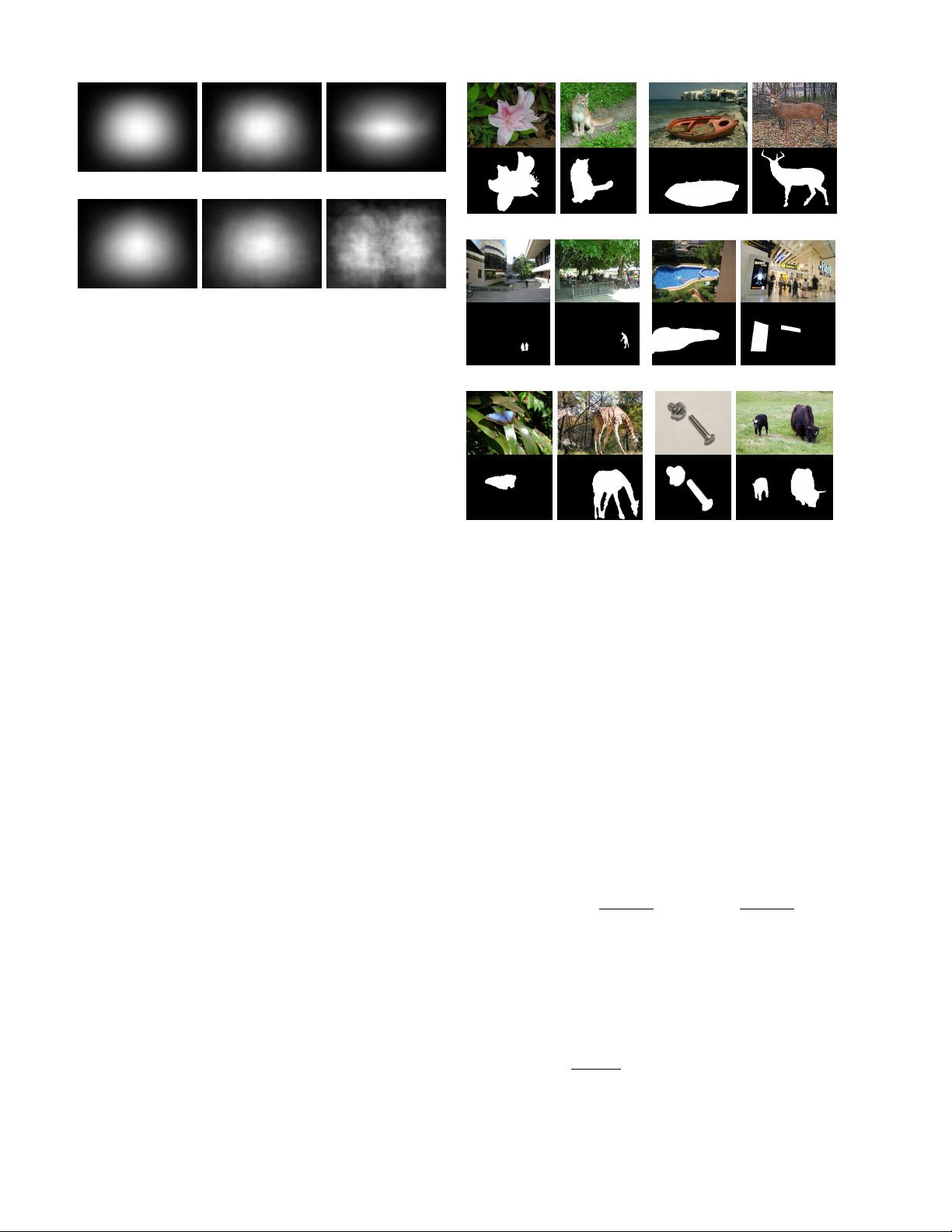
(a) MSRA10K (b) ECSSD (c) THUR15K

(d) DUT-OMRON (e) JuddDB (f) SED2

Fig. 2. Average annotation maps of six datasets used in benchmarking.

images in SED2 usually have two objects aligned around

opposite image borders. Moreover, we can see that the

spatial distribution of salient objects in JuddDB has a larger

variety than other datasets, indicating that this dataset have

smaller positional bias (i.e., center-bias of salient objects

and border-bias of background regions).

In Fig. 4(b), we aim to show the complexity of images

in six benchmark datasets. Toward this end, we apply the

segmentation algorithm by Felzenszwalb et al. [101] to see

how many super-pixels (i.e., homogeneous regions) can be

obtained on average from salient objects and background

regions of each image, respectively. In this manner, we can

use this measure to reﬂect how challenging a benchmark

is since massive super-pixels often indicate complex fore-

ground objects and cluttered background. From Fig. 4(c),

we can see that JuddDB is the most challenging benchmark

since it has an average number of 493 super-pixels from the

background of each image. On the contrary, SED2 contains

fewer number of super-pixels in foreground and background

regions, indicating that images in this benchmark often

contain uniform regions and are easy to process.

In Fig. 4(c), we demonstrate the average object sizes

of these benchmarks, while the size of each object is

normalized by the size of the corresponding image. We

can see that MSRA10K and ECCSD datasets have larger

objects while SED2 has smaller ones. In particular, we

can see that some benchmarks contain a limited number

of image regions with large foreground objects. By jointly

considering the center-bias property, it becomes very easy

to achieve a high precision on these images.

C. Evaluation Measures

There are several ways to measure the agreement be-

tween model predictions and human annotations [21]. Some

metrics evaluate the overlap between a tagged region while

others try to assess the accuracy of drawn shapes with

object boundary. In addition, some metrics have tried to

consider both boundary and shape [102].

Here, we use three universally-agreed, standard, and

easy-to-understand measures for evaluating a salient object

detection model. The ﬁrst two evaluation metrics are based

on the overlapping area between subjective annotation and

(a) MSRA10K (b) ECSSD

(e) THUR15K (f) SED2

Fig. 3. Images and pixel-level annotations from six salient object datasets.

saliency prediction, including the precision-recall (PR) and

the receiver operating characteristics (ROC). From these

two metrics, we also report the F-Measure, which jointly

considers recall and precision, and AUC, which is the area

under the ROC curve. Moreover, we also use the third

measure which directly computes the mean absolute error

(MAE) between the estimated saliency map and ground-

truth annotation. For the sake of simpliﬁcation, we use S to

represent the predicted saliency map normalized to [0, 255]

and G to represent the ground-truth binary mask of salient

objects. For a binary mask, we use | · | to represent the

number of non-zero entries in the mask.

Precision-recall (PR). For a saliency map S, we can

convert it to a binary mask M and compute P recision

and Recall by comparing M with ground-truth G:

P recision =

|M ∩ G|

|M|

, Recall =

|M ∩ G|

|G|

(1)

From this deﬁnition, we can see that the binarization

of S is the key step in the evaluation. Usually, there are

three popular ways to perform the binarization. In the ﬁrst

solution, Achanta et al. [18] proposed the image-dependent

adaptive threshold for binarizing S, which is computed as

twice as the mean saliency of S:

W × H

x=1

y=1

S(x, y), (2)

where W and H are the width and the height of the saliency

map S, respectively.

The second way to bipartite S is to use a ﬁxed threshold

which changes from 0 to 255. On each threshold, a pair

剩余15页未读，继续阅读

chent1995

粉丝: 2
资源: 7

2015年IEEE Transactions on Image Processing论文：视觉显著对象检测基准研究

RGBD Salient Object Detection A Benchmark and Algorithms

ECSSD 显著度图 of Deeply Supervised Salient Object Detection with Short Connections

Deeply Supervised Salient Object Detection with Short Connections在自己数据集上训练（tensorflow版本）-附件资源

UFO_Salient_Region_Detection原稿_salient_ufo_

matlab代码影响-salient_object_detection_evaluation:显着物体检测评估

CVPR2007_Learning_to_detect_a_salient_object

matlab代码影响-salient_object_distribution:Matlab脚本来分析图像中显着对象的空间分布

MINet-master_salientobject_scale_

salient_map

Saliency-Extraction-master_least3do_salient_saliency_contrast_fi

最新资源