五维爱因斯坦-高斯-贝内特引力下的各向异性紧凑星研究
PDF格式 | 1.34MB |
更新于2024-09-03
| 24 浏览量 | 举报
"这篇文章探讨了五维爱因斯坦-高斯-贝内特引力理论下各向异性紧凑星的性质,研究中采用了Tolman-Kuchowicz时空模型,并通过耦合常数α来考察其对物质分布的影响。"
本文是开放获取的学术文章,发布在《欧洲物理杂志C》上,探讨了在五维爱因斯坦-高斯-贝内特引力理论背景下的各向异性致密物质分布。爱因斯坦-高斯-贝内特(Einstein-Gauss-Bonnet, EGB)引力是广义相对论的一种扩展,它引入了一个额外的高斯-邦内拉格朗日项(Gauss-Bonnet Lagrangian, LGB),这个项通过耦合常数α与爱因斯坦-希尔伯特作用相关联。当耦合常数α趋近于零时,理论退化为标准的广义相对论。
为了研究这个理论下的物质分布,作者选择了Tolman-Kuchowicz时空作为内部几何模型,该模型能够描述具有各向异性的物质分布。作者分析了耦合常数α对模型关键特性的影响,如能量密度、径向压力、切向压力以及各向异性因子。通过对比这些参数与广义相对论的结果,揭示了EGB引力中独特的物理现象。
此外,作者还研究了稳定性的条件,即通过广义的Tolman-Oppenheimer-Volkoff(TOV)方程来实现物质的静态平衡,并利用相对论绝热指数和Abreu准则来评估模型的稳定性。同时,通过因果条件和能量条件分析了压力波在恒星结构主要方向上的传播速度,以及整个能量动量张量的传导特性。
文章通过数学、物理和图形化的手段详细阐述了这些主题。M-I(Mass-Interior)和M-R(Mass-Radius)图表明,随着α的增加,状态方程的刚度增强,但其刚度仍小于广义相对论情况。这些发现提供了关于EGB引力中紧凑星可能行为的新洞察,为理解和探索高维引力理论提供了重要的理论依据。
这篇论文为理解五维EGB引力下的紧凑星物理性质提供了深入的理论研究,对于未来的引力理论研究以及天体物理学的实践应用具有重要意义。
Eur. Phys. J. C (2019) 79 :922 Page 3 of 12 922
G
μν
= R
μν
−
R
2
g
μν
, (4)
H
μν
= 2
RR
μν
− 2R
μω
R
ω
ν
− 2R
ωβ
R
μωνβ
+R
ωβ γ
μ
R
νωβγ
−
1
2
g
μν
L
GB
. (5)
The energy-momentum tensor T
μν
corresponding to the mat-
ter fields is obtained from S
matter
.
So, by taking n = 5, the five-dimensional line element
for a static spherically symmetric spacetime has the standard
form
ds
2
=−e
2ν(r)
dt
2
+ e
2λ(r)
dr
2
+r
2
(dθ
2
+ sin
2
θ dφ
2
+sin
2
θ sin
2
φdψ
2
), (6)
in coordinates (x
i
= t, r,θ,φ,ψ). For our model the energy-
momentum tensor for the stellar fluid is taken to be
T
μν
= diag
(
−ρ, p
r
, p
t
, p
t
, p
t
)
, (7)
where ρ, p
r
, and p
t
are the proper energy density, the radial
pressure, and the tangential pressure, respectively. By con-
sidering the comoving fluid velocity as u
a
= e
−ν
δ
a
0
,theEGB
field equation (3) leads to the following set of independent
equations:
κρ =
3
e
4λ
r
3
4αλ
+re
2λ
−re
4λ
−r
2
e
2λ
λ
− 4αe
2λ
λ
,
(8)
κp
r
=
3
e
4λ
r
3
(r
2
ν
+r + 4αν
)e
2λ
−re
4λ
− 4αν
, (9)
κp
t
=
1
e
4λ
r
2
12αν
λ
− e
4λ
− 4αν
− 4αν
2
+
1
e
2λ
r
2
1 − r
2
ν
λ
+ 2rν
− 2rλ
+r
2
ν
2
+
1
e
2λ
r
2
r
2
ν
− 4αν
λ
+ 4αν
2
+ 4αν
. (10)
Besides, we have considered units such that the speed of light
c and the constant G
5
are set to unity. Then κ = 8π.Here
denotes differentiation with respect to the radial coordinate
r.
3 Solution of the field equations
To solve the above field equations (8)–(10) we choose λ(r) =
ln(1 + ar
2
+ br
4
) and ν = Br
2
+ 2lnC with a, b, B and
C as constants. These metric potentials conform to the well-
known Tolman–Kuchowicz [43,44] spacetime. This choice
on e
λ
and e
ν
is well motivated because both metric potentials
are free from physical and mathematical singularities at every
point inside the compact star. Moreover, at the center of the
structure they have the appropriate behavior, i.e., e
λ(r)
|
r=0
=
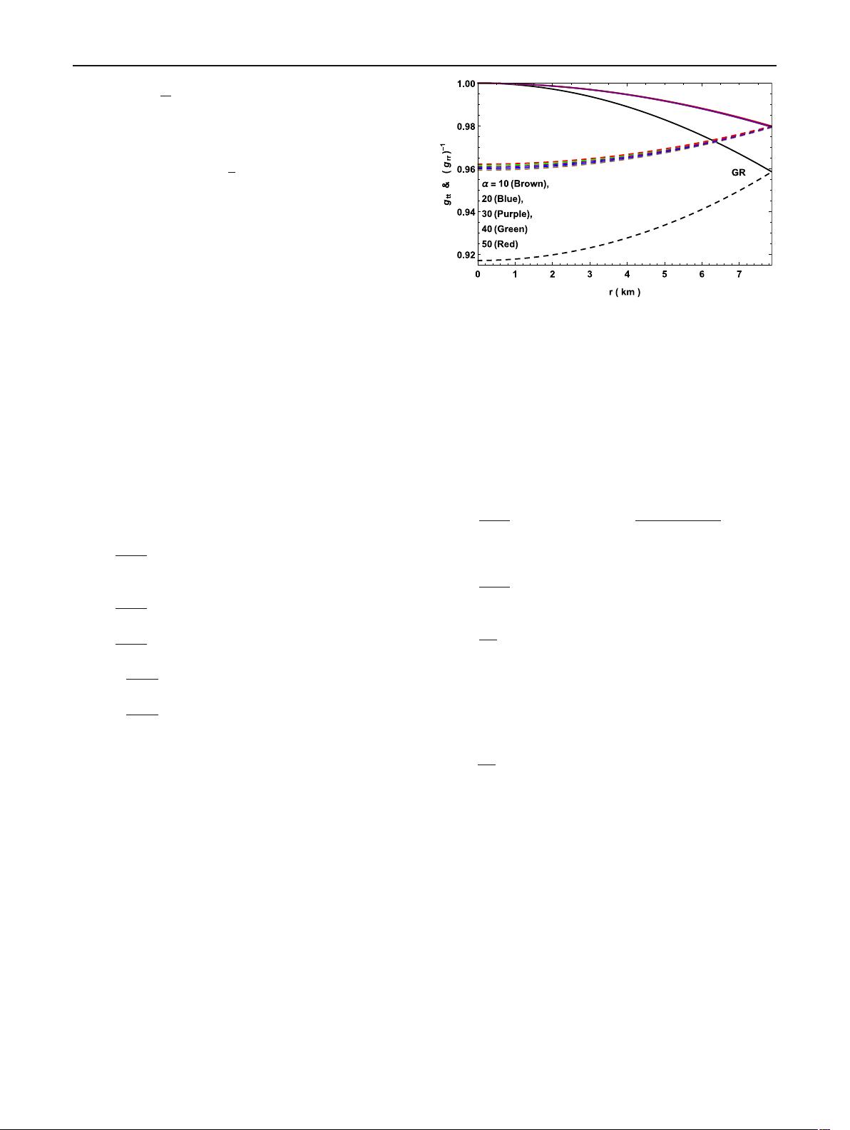
Fig. 1 Variation of metric potentials for 4U 1538-52 using the param-
eter provided in Table 1
1 and e
ν(r)
|
r=0
= C
2
, which implies (e
λ
)
|
r=0
= (e
ν
)
|
r=0
=
0, as is required for a well behaved model. The trend of the
inner geometry is displayed in the upper panel of Fig. 1.
A completely regular behavior is observed, also as α grows
e
λ
and e
ν
take higher values, in distinction with GR whose
values are dominated by those of EGB theory for all r. So,
inserting e
λ
and e
ν
into Eqs. (8)–(10)wearriveat
κρ =
3
r
3
4
8αr (a + 2br
2
) −
8αr (a + 2br
2
)
+2r
3
(a + 2br
2
) −r
2
+r
4
)
, (11)
κp
r
=
3
r
3
4
(r + 8αBr + 2Br
3
)
2
− 8α Br − r
4
,
(12)
κp
t
=
1
5
48α B(a + 2br
2
) + 8α B(a − 2B + br
2
)
−4
a − 2B + 2aα B + B
1
r
2
2
− (a + br
2
)
4
−
3
a + 2B + br
2
− 4B
2
(4α + r
2
)
. (13)
The anisotropic factor defined by ≡ p
t
− p
r
is obtained:
κ =
2
5
24α B(a + 2br
2
) − 8α B(a + B + br
2
)
−2(a − 2B + 8aα B + B
2
r
2
)
2
+ (a + br
2
)
4
+
3
a + br
2
+ 2B(−2 + 4α B + Br
2
)
(14)
where
B
1
=−aB + b(2 + 6α B),
= (1 + ar
2
+ br
4
),
B
2
=−aB + 2b(1 + 6α B).
The behavior of the metric function, density, pressure,
anisotropy and equation of state parameter are given in Figs.
1, 2, 3, 4 and 5. The interior red-shift can be found to be
z(r) = e
−ν/2
− 1 (15)
123
剩余11页未读,继续阅读
相关推荐

168 浏览量

weixin_38651507
- 粉丝: 1
 我的内容管理
展开
我的内容管理
展开


最新资源
- 普天身份证阅读器新版二次开发包发布
- C# 实现文件的数据库保存与导出操作
- CkEditor增强功能:轻松实现图片上传
- 掌握DLL注入技术:测试工具使用与探索
- 实现带节假日农历功能的jQuery日历选择器
- Spring循环依赖示例:深入理解与Git代码仓库实践
- ABB PLC液压阀门控制程序开发指南
- 揭秘4核旋风密版626象棋引擎的超牛实力
- HTML5实现的经典游戏:小霸王坦克大战源码分享
- 让Visual Studio兼容APM硬件信息的方法
- Kotlin入门:创建我的第一个应用
- Android语音识别技术研究报告与应用分析
- 掌握JavaScript基础:第8版教程源代码解析
- jQuery制作动态侧面浮动图片广告特效教程
- Android PinView仿支付宝密码输入框源码分析
- HTML5 Canvas制作的围住神经猫游戏源码分享
