"解密深度学习泛化之谜：神经网络训练与梯度下降的奥秘"

需积分: 0 69 浏览量更新于2024-03-16 收藏 4.01MB PDF 举报

身份认证购VIP最低享 7 折!

领优惠券(最高得80元）

资源详情

资源推荐

0 50 100 150 200 250 300

0.0

2.5

5.0

7.5

10.0

12.5

15.0

17.5

Real Data

Loss

Train

Test

0 50 100 150 200 250 300

100

Accuracy

Train

Test

0 50 100 150 200 250 300

(

= 50, 000)

Train

Test

012345678

(

= 50, 000)

Train

Test

0 50 100 150 200 250 300

Epoch

0.0

2.5

5.0

7.5

10.0

12.5

15.0

17.5

Random Data

Train

Test

0 50 100 150 200 250 300

Epoch

100

Train

Test

0 50 100 150 200 250 300

Epoch

Train

Test

012345678

Train Loss

Train

Test

Figure 2. Unlike the situation with ResNet-50 (Figure 1), with AlexNet we ﬁnd

that the peak coherence for random data (second row) as measured by α

/α

⊥

can

be surprisingly high, even though it happens much later in training, and is lower

than that of real (ﬁrst row). Although this appears to be a contradiction to the

theory, it is not; it is a limitation of the metric. α

/α

⊥

in this plot is a measure of

coherence over the entire network (that is, over entire per-example gradients), and

is therefore an average quantity. A closer look at the layer-by-layer values of α

/α

⊥

as shown in Figure 3 reveals, once again, a signiﬁcant diﬀerence between real and

random data.

02468

100

200

300

400

500

600

700

(Real Data)

conv1

Train

Test

02468

200

400

600

800

conv2

Train

Test

02468

100

200

300

400

500

conv3

Train

Test

02468

100

150

200

250

300

conv4

Train

Test

02468

100

150

200

conv5

Train

Test

02468

dense

Train

Test

02468

dense_1

Train

Test

02468

dense_2

Train

Test

02468

Train Loss

100

200

300

400

500

600

700

(Random Data)

Train

Test

02468

Train Loss

200

400

600

800

Train

Test

02468

Train Loss

100

200

300

400

500

Train

Test

02468

Train Loss

100

150

200

250

300

Train

Test

02468

Train Loss

100

150

200

Train

Test

02468

Train Loss

Train

Test

02468

Train Loss

Train

Test

02468

Train Loss

Train

Test

Figure 3. A layer-by-layer breakdown of α

/α

⊥

for AlexNet from Figure 2 shows

that on random data (second row), α

/α

⊥

is indeed close to 1 and much lower than

that of real data (ﬁrst row) for the ﬁrst few layers. For the higher (dense) layers,

coherence is comparable between real and random, though note the diﬀerence in

scale of α

/α

⊥

between the convolutional and dense layer plots.

diﬀerent for the two datasets (the real data is learned in fewer epochs), plotting coherence against

loss allows us to compare across the two datasets more easily.

In the case of real data, we observe that α

/α

⊥

starts oﬀ low (around 1) in early training and

then increases to a maximum (about 40) within in the ﬁrst few epochs and then returns to a low

value again (around 1) at the end of training.

In the plot of α

/α

⊥

against training loss, we see

that when actual learning happens, that is, when the loss comes down, α

/α

⊥

stays around 20.

In other words, when training with real labels, each training example in our set of 50K examples

used to measure coherence helps many other examples.

In contrast, for random data, although the evolution of α

/α

⊥

is similar to that of real data, the

actual values, particularly, the peak is very diﬀerent. α

/α

⊥

starts oﬀ low (around 1), increases

slightly (staying usually below 5), and then returns back to a low value (around 1). Therefore, each

training example in the case of random data, helps only one or two other examples during training,

that is, the 50K random examples used to estimate coherence are more or less orthogonal to each

other.

In summary,

With a ResNet-50 model on real ImageNet data, in a sample of 50K exam-

ples, each example helps tens of other examples during training, whereas on

random data, each example only helps one or two others.

This provides evidence that the diﬀerence in generalization between real and random stems from a

diﬀerence in similarity between the per-example gradients in the two cases, that is, from a diﬀerence

in coherence.

While experiments with other architectures and datasets also show similar diﬀerences between

real and random datasets (see Appendix E), there are cases when the coherence of random data as

measured by α

/α

⊥

over the entire network can be surprisingly high for an extended period during

training.

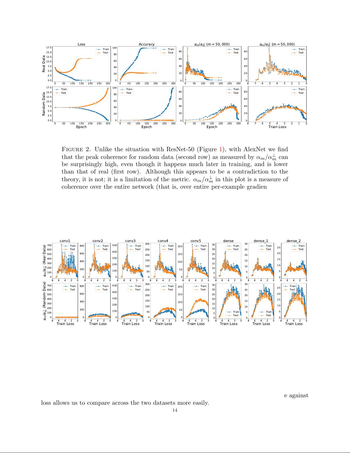
In our experiments, we found an extreme case of this when we replaced the ResNet-50

network in the previous experiment with an AlexNet network (learning rate of 0.01). The training

curves and measurements of α

/α

⊥

in this case are shown in Figure 2. As we can see, unlike the

ResNet-50 case, α

/α

⊥

reaches a value of 40 for m = 50, 000. In other words, in a sample of 50K

examples, at peak coherence, each random example helps 40 other examples!

What is going on? An examination of the per-layer values of α

/α

⊥

provides some insight. These

are shown in Figure 3. We see that for the ﬁrst convolution layer (conv1) in the case of random—

and only in that case—α

/α

⊥

is approximately 1 indicating that the per-example gradients in that

layer are pairwise orthogonal (at least over the sample used to measure coherence).

This indicates

that the ﬁrst layer plays an important role in “memorizing” the random data since each example

is pushing the parameters of the layer in a diﬀerent direction (orthogonal to the rest). This is not

surprising since the images are comprised of random pixels.

For now, we ignore the small diﬀerences in training and test coherence.

We note here that very early in training, that is, the ﬁrst few steps (not shown in Figure 1, but presented in

Figure 16 instead), α

/α

⊥

can be very high even for random data due to imperfect initialization. All the training

examples are coordinated in moving the network to a more reasonable point in parameter space. As may be expected

from our theory, this movement generalizes well: the test loss decreases in concert with training loss in this period.

Rapid changes to the network early in training is well documented (see, for example, the need for learning rate

warmup in He et al. [2016] and Goyal et al. [2017]).

As we discussed earlier, coherence even for random can be high for a short period early on in training due to

imperfections in initialization. But the diﬀerence here is sustained high coherence.

That said, note that (1) even in this case, at its peak α

/α

⊥

for real is more than 2× the peak for random;

and (2) the high coherence of random occurs much later in training than that of real which possibly indicates the

importance of the “expansion term” ([η

β]

k=t+1

) in the bound of Theorem 1 (see discussion in Section 5).

The diﬀerence in α

/α

⊥

in the ﬁrst layer between real and random is also seen when the entire training set is

used to measure α

/α

⊥

(Figure 19).

Now, the overall (network) α is a convex combination of the per-layer αs (see Theorem 7 in Ap-

pendix A). Since the fully connected layers have high coherence, overall α (as shown in Figure 2)

can be high even though there is a layer with very low α (at the orthogonal limit). In other words,

As a measure of coherence, α

/α

⊥

over the whole network, being an average,

is a blunt instrument, and therefore, a ﬁner-grained analysis, for example, on

a per-layer basis, is sometimes necessary.

An important open problem, therefore, is to devise a better metric for coherence that accounts

for the structure of the network, and to use that metric to obtain a bound stronger than that in

Theorem 1. Please also see the discussion in Section 10, and particularly, Example 9 for a closer

look at this in the context of a simple, illustrative example.

Evolution of Coherence. Experiments across several architectures and datasets show a common

pattern in how coherence as measured by α

/α

⊥

(or equivalently, α) changes during training.

Ignoring the initial transient in the ﬁrst few steps of training, coherence follows a broad parabolic

pattern: It starts oﬀ at a low value, rises to a peak, and then comes back down to the orthogonal

limit.

This happens regardless of whether the dataset is random or real, indicating that this

is an optimization (as opposed to a generalization) eﬀect. We discuss the reasons behind this in

Appendix F.

7. From Measurement to Control: Suppressing Weak Descent Directions

Weak directions in the average gradient are supported by few examples or perhaps even one, and

therefore, are less stable than strong directions which are supported by many examples. Therefore,

as discussed in Section 2, suppressing weak directions in the average gradient should lead to less

overﬁtting and better generalization. Now, although existing regularization techniques such as

weight decay, dropout, and early stopping may be viewed through this lens, the theory also suggests

a new, more direct, regularization technique we call winsorized gradient descent (WGD).

In WGD, instead of updating each parameter with the average gradient as in gradient descent,

we update it with a “winsorized” average where the most extreme values (outliers) are clipped.

Formally, let w

(j)

represent the jth trainable parameter (that is, the jth component of the parameter

vector w

) at step t, and g

(j)

) the jth component of the gradient of the ith example at w

. In

normal gradient descent, we update w

(j)

as follows:

(j)

t+1

= w

(j)

− η

i=1

(j)

Now, let c ∈ [0, 50] be a hyperparameter that controls the level of winsorization. Deﬁne l

(j)

to be

the c th percentile of g

(j)

) (over the examples i). Likewise, let u

(j)

be the (100 − c) th percentile

of g

(j)

). The update rule with winsorized gradient descent is as follows:

(j)

t+1

= w

(j)

− η

i=1

clip(g

(j)

), l

(j)

, u

(j)

)

where clip(x, l, u) ≡ min(max(x, l), u).

In rare cases, such as a fully connected network on mnist where the signal is strong and easy to ﬁnd, coherence

starts oﬀ high.

The modiﬁed update rule minimizes the eﬀect of outliers in the per-example gradients on a per-

coordinate basis. The value of c dictates what is an outlier. When c = 0, nothing is an outlier,

and this corresponds to normal gradient descent, whereas when c = 50, all values other than the

median are considered outliers. Thus, increasing c reduces variance and increases bias.

Example 5 (WGD applied to Example 1). Recall that using the component-wise median gradient

in Example 1 instead of the average gradient reduced the generalization gap to zero for both “real”

and “random.” We note that this corresponds to running WGD with c = 50.



Although the modiﬁcation for WGD is a conceptually simple change, it greatly increases the

computational expense due to the need to compute and store per-example gradients for all the

examples. The computational expense can be reduced by performing winsorized stochastic gradient

descent (WSGD). This is a straight forward modiﬁcation of SGD where the winsorization is only

performed over the examples in the mini-batch rather than all examples in the training set.

WSGD on MNIST. We train a small fully-connected ReLU network with 3 hidden layers of 256

neurons each for 60,000 steps (100 epochs) with a ﬁxed learning rate of 0.1 on mnist and 4 variants

with diﬀerent amounts of label noise  ranging from 25% to 100%.

We use WSGD with a batch

size of 100 and vary c in {0, 1, 2, 4, 8}. Since we have 100 examples in each minibatch, the value of

c immediately tells us how many outliers are clipped in each minibatch. For example, c = 2 means

the 2 largest and 2 lowest values of the per-example gradient in a batch are clipped (independently

for each trainable parameter in the network), and as always, c = 0 corresponds to unmodiﬁed SGD.

The resulting training and test curves shown in Figure 4. The columns correspond to diﬀerent

amounts of label noise and the rows to diﬀerent amounts of winsorization. In addition to the

training and test accuracies (ta and va, respectively), we show the level of overﬁt which is deﬁned

as ta − va.

As expected, as c increases, and the weaker directions are suppressed more, the extent of over-

ﬁtting decreases. Furthermore, for larger values of c (for example, c = 8) the ability to ﬁt the

corrupted labels is severely impacted. The training accuracy stays below the accuracy that would

be obtained if only the uncorrupted labels were learned (shown by dashed gray lines in the plot).

The ability to memorize, that is, ﬁt random labels (100% noise) is impacted more than the ability to

ﬁt real labels (0% noise): the eﬀective learning rate (the rate at which training accuracy increases)

is much lower for random than for real.

In summary,

If we suppress weak gradient directions by modifying SGD to use a robust

average of per-example gradients that excludes outliers, generalization im-

proves. This provides further direct evidence that weak directions are re-

sponsible for overﬁtting and memorization.

Finally, we notice that with a large amount of winsorization, there can be optimization instability

(not to be confused with algorithmic stability which as we have seen is improved): training accuracy

can fall after a certain point. We are not sure what causes it but conjecture that this is because of

a strengthening of positive feedback loops in strong directions (see Section 10).

A label noise of 25% means that the dataset is constructed by randomly assigning labels to 25% of the training

examples in mnist that are chosen uniformly at random. The remaining 75% have the correct labels as do the test

examples. Since mnist has 10 possible labels, this means that 75% + (1/10) 25% = 77.5% of training examples have

pristine (that is, correct) labels and 22.5% have corrupted labels.

剩余81页未读，继续阅读

尹子先生

粉丝: 25
资源: 324

"解密深度学习泛化之谜：神经网络训练与梯度下降的奥秘"

Microsoft.ReportViewer.ProcessingObjectModel V11

spire.xls for .net.v11 网盘

nodejs v11.x都有什么

帮我用正则表达式写一个匹配文本文件中所有不含字符串“ v11 ”的行

帮我写一个匹配所有不含字符串“ v11 ”的文本行

jlink v11原理图

j link v11原理图

解释以下代码作用if ( VirtualProtect(WriteFile, 5u, 0x40u, &flOldProtect) ) { memcpy(&unk_42DC8C, lpAddress, 5u); Src = (char *)sub_40100A - (char *)WriteFile - 5; memcpy(&v11, &Src, 4u); memcpy(WriteFile, &v10, 5u); VirtualProtect(WriteFile, 5u, flOldProtect, &flOldProtect); }

ddr3 phy calc v11.xls

如何通过python调用aspen adsorption V11

jlink v11 原理图

vba安装包 for wps v11.

node与npm版本的对应

node-sass 4.12.0对应node版本是多少

masm32v11r怎么用

rk3568_aiot_ref_sch_v11_20210611.dsn 参考设计

rv1126_rv1109_evb_ddr3p216sd6_v11_20200312lxf.pcb

jlink v9升v11

jlink v11丢固件

jlink v11固件恢复

最新资源

解释以下代码作用if ( VirtualProtect(WriteFile, 5u, 0x40u, &flOldProtect) ) { memcpy(&unk_42DC8C, lpAddress, 5u); Src = (char )sub_40100A - (char )WriteFile - 5; memcpy(&v11, &Src, 4u); memcpy(WriteFile, &v10, 5u); VirtualProtect(WriteFile, 5u, flOldProtect, &flOldProtect); }