
Le
Lw
o
i
~{Q
0
(v
o
)y
h
i
,
ð11Þ
where
Q
0
(v)~a(1{tanh
2
(avzb))~a(1{y
2
):
In a multi-layer FNN, a backpropagation algorithm is usually used
to train the weight matrix from the input layer to the hidden layer,
W
h
. If the EEC cost function is used, the training algorithm is the
MEE algorithm [22]. The derivative of the error e with respect to
the weight w
h
k,l
in the matrix W
h
can be calculated as
Le
Lw
h
k,l
~{Q
0
(v
o
)w
o
k
Q
0
(v
h
k
)u
l
:
ð12Þ
By Eq. (11) and Eq. (12), the weight update rule in Eq. (7) and Eq.
(8) can be calculated.
On the basis of the algorithm description in [23], the proposed
synergistic learning algorithm for the FNN is summarized as
follows:
Step 1. Initialization. Choose a random set of small values
for the P|M hidden layer weight matrix W
h
and the M|1
output layer weight matrix W
o
. Set a~1 and b~0 for each
neuron. Let u(n)~½u
1
(n),u
2
(n), ...,u
P
(n)
T
be the input signal and
let d(n) be the corresponding desired network output. The number
of samples in the training set is n
0
, thus 1ƒnƒn
0
.
Step 2. Repetition. The epochwise training procedure begins
with n~1. Repeat the following calculations with the input vector
u(n) and the target output d(n) for 1ƒnƒn
0
v
h
(n) ~(W
h
)
T
u(n),
y
h
(n) ~Q
h
(v
h
(n)),
v
o
(n) ~(W
o
)
T
y
h
(n),
y
o
(n) ~Q
o
(v
o
(n)),
e(n) ~d(n){y
o
(n),
ð13Þ
where
v
h
(n) ~½v
h
1
(n),v
h
2
(n), ...,v
h
M
(n)
T
,
Q
h
(v
h
(n))
~½Q
h
1
(v
h
1
(n); a
1
,b
1
),Q
h
2
(v
h
2
(n); a
2
,b
2
), ...,
Q
h
M
(v
h
M
(n); a
M
,b
M
)
T
,
y
h
(n) ~½y
h
1
(n),y
h
2
(n), ...,y
h
M
(n)
T
:
Step 3. Weight Matrix Update. Update the weight matrices
W
o
and W
h
by the weight update algorithm. Calculation results of
v
k
(n) and y
k
(n) in Eq. (13) are used to compute the derivatives of
the error with respect to the weight in Eq. (11) and Eq. (12); with
the results of the derivatives and the errors e(n) in Eq. (13), Eq. (8)
can be computed and finally the weight matrices can be updated
by Eq. (7).
Step 4. Activation Function Update. Update the parame-
ters a
k
and b
k
of the activation function Q
k
of the neuron k using
the intrinsic plasticity rule described in Eq. (2) with all values of
v
k
(n) and y
k
(n). By the batch version of the IP rule, the
parameters a
k
and b
k
are only updated once during an epoch.
Step 5. Return or Stop. If the stopping criterion is satisfied,
the training procedure is stopped; otherwise, set n~1 and return
to Step 2.
Construction of the RNN
In this section, we continue to study the proposed synergistic
learning algorithm in a general class of recurrent neural networks
[23,24]. As illustrated in Fig. 2, the neural network contains N
neurons. The input vector u is comprised of the external signal
vector of P elements ½u
1
,u
2
, ...,u
P
T
, and the feedback vector
r~½r
1
,r
2
, ...,r
N
T
. The feedback signal r
k
after a delay of one
time unit is the output of the kth neuron y
k
, r
k
(n)~y
k
(n{1), thus
the feedback vector at the time point n can be rewritten as
r(n)~½y
1
(n{1),y
2
(n{1), ...,y
N
(n{1)
T
. Then the input vector
at the time point n is given by
u(n)~½u
1
(n),u
2
(n), ...,u
P
(n),y
1
(n{1),y
2
(n{1), ...,y
N
(n{1)
T
:
The (Pz1zN)|N synaptic weight matrix of the recurrent
network is represented by W. An element w
k,l
of this matrix
represents the connection weight from the lth input node to the
kth neuron. With the input vector u and the activation function Q,
the N|1 output vector y~½y
1
,y
2
, ...,y
N
is calculated as
v ~W
T
u,
y ~Q(v),
ð14Þ
where v~½v
1
,v
2
, ...,v
N
and y
1
is the single output of the network.
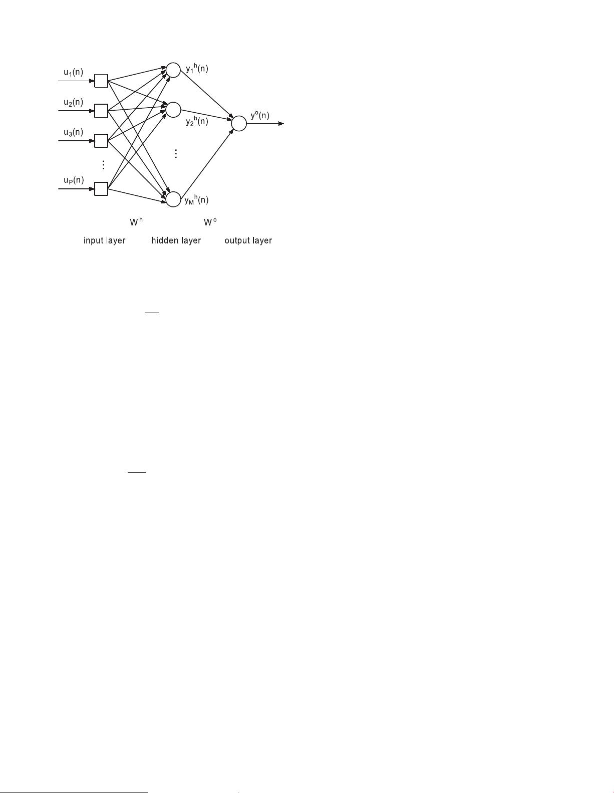
Figure 1. Structure of the feedforward neural networks.
doi:10.1371/journal.pone.0062894.g001
Synergistic Learning Based on Information Theory
PLOS ONE | www.plosone.org 4 May 2013 | Volume 8 | Issue 5 | e62894
剩余16页未读,继续阅读

weixin_38553681
- 粉丝: 2
- 资源: 915
 我的内容管理
展开
我的内容管理
展开


最新资源
- OptiX传输试题与SDH基础知识
- C++Builder函数详解与应用
- Linux shell (bash) 文件与字符串比较运算符详解
- Adam Gawne-Cain解读英文版WKT格式与常见投影标准
- dos命令详解:基础操作与网络测试必备
- Windows 蓝屏代码解析与处理指南
- PSoC CY8C24533在电动自行车控制器设计中的应用
- PHP整合FCKeditor网页编辑器教程
- Java Swing计算器源码示例:初学者入门教程
- Eclipse平台上的可视化开发:使用VEP与SWT
- 软件工程CASE工具实践指南
- AIX LVM详解:网络存储架构与管理
- 递归算法解析:文件系统、XML与树图
- 使用Struts2与MySQL构建Web登录验证教程
- PHP5 CLI模式:用PHP编写Shell脚本教程
- MyBatis与Spring完美整合:1.0.0-RC3详解
资源上传下载、课程学习等过程中有任何疑问或建议,欢迎提出宝贵意见哦~我们会及时处理!
点击此处反馈


