CHEN et al.: DEEP FEATURE EXTRACTION AND CLASSIFICATION OF HYPERSPECTRAL IMAGES 6235
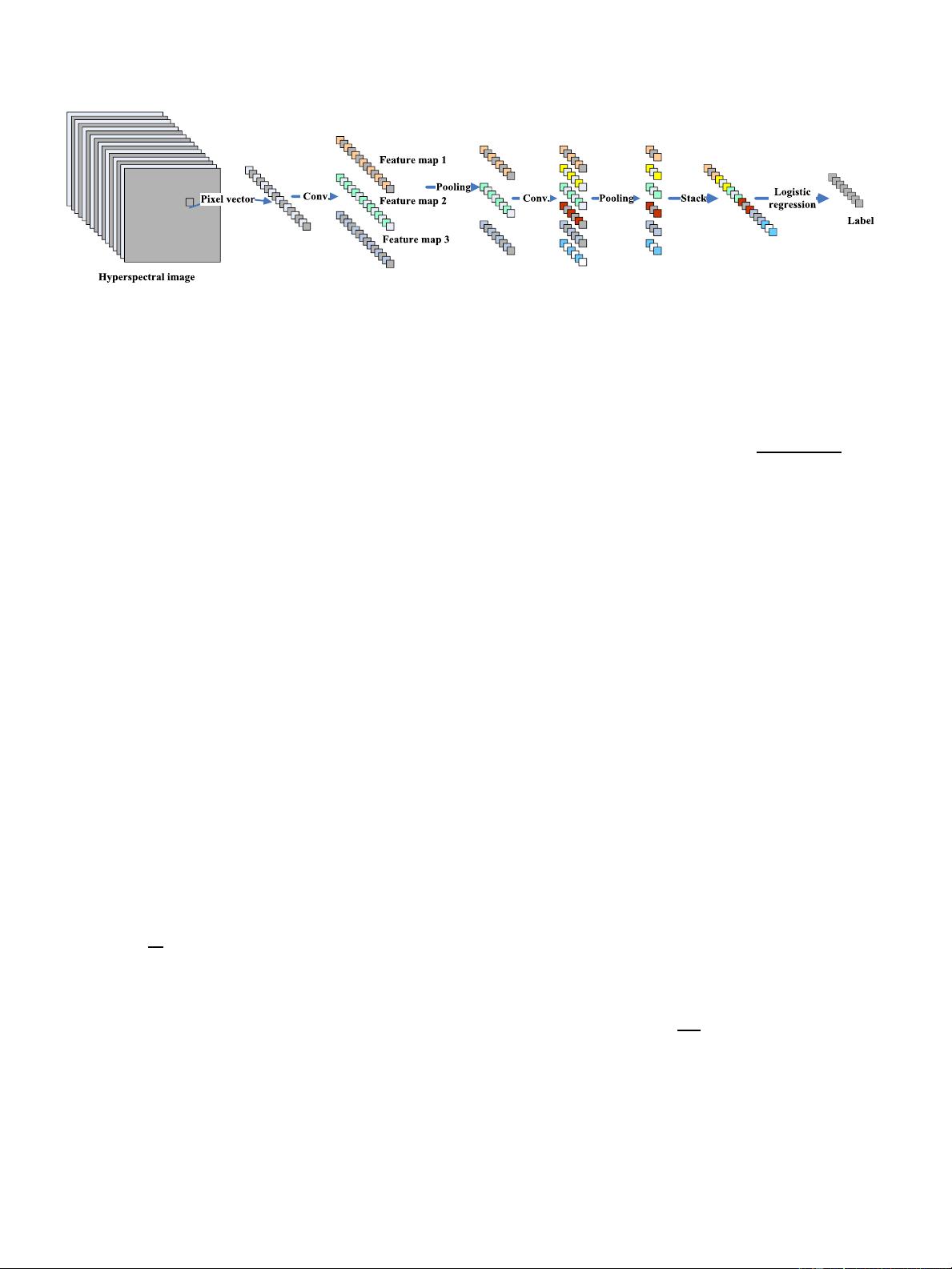
Fig. 3. Architecture of deep CNN with spectral FE of HSI.
and classification. In the FE p rocedure, LR is taken into account
to adjust the weights and biases in the back-propagation. After
the training, the learned features can be used in conjunction
with classifiers such as LR, K-nearest neighbor (KNN), and
SVMs [1].
The proposed architecture is shown in Fig. 3. The input of the
system is a pixel vector of hyperspectral data, and the output of
the system is the label of the pixel vector. It consists of several
convolutional and pooling layers and an LR layer. In Fig. 3, as
an example, the flexible CNN model includes two convolution
layers and two pooling layers. There are three feature m aps in
the first convolution layer and six feature maps in the second
convolution layer.
After several layers of convolution and pooling, the in-
put pixel vector can be converted into a feature vector,
which captures the spectral information in the input pixel
vector. Finally, we use LR or other classifiers to fulfill the
classification step.
The power of CNN depends on the connections (weights) of
the network; hence, it is very important to find a set of proper
weights. Gradient back-propagation is the core fundamental
algorithm for all kinds of neural networks. In this paper, the
model parameters are initialized randomly and trained by an
error back-propagation algorithm.
Before setting an updating r ule for the weights, one needs
to properly set an “error” measure, i.e., a cost function. There
are several ways to define such a cost function. In our imple-
mentation, a mini-batch update strategy is adopted, which is
suitable for large data set processing, and the cost is computed
on a mini-batch of inputs [37]
c
0
= −
1
m
m
i=1
[x
i
log(z
i
)+(1− x
i
) log(1 − z
i
)] . (4)
Here, m denotes the mini-batch size. Two variables x
i
and
z
i
denote the ith predicted label and the label in the mini-
batch, respectively. The i summation is done over the whole
mini-batch. Our hope turns to optimize (4) using mini-batch
stochastic gradient descent.
LR is a type of probabilistic statistical classification model.
It measures the relation b etween a categorical variable and the
input variables using probability scores as the predicted values
of the input variables.
To pe rform classificatio n b y utilizing the learned features
from the CNN, we employ an LR classifier, which uses soft-
max as its output-layer activation. Softmax ensures that the
activation of each output unit sums to 1 so that we can deem
the output as a set of conditional probabilities. For given input
vector R, the probability that the input belongs to category i can
be estimated as follows:
P (Y = i|R, W, b)=s(WR+ b)=
e
W
i
R+b
i
j
e
W
j
R+b
j
(5)
where W and b are the weights and biases of the LR layer, and
the summation is done over all the output units.
In the LR, the size of the output layer is set to be the same
as the total number of classes defined, and the size of the input
layer is set to be the same as the size of the output layer of
the CNN. Since the LR is implemented as a single-layer neural
network, it can be merged with the former layers of networks to
form a d eep classifier.
D. L2 Regularization of CNN
Overfitting is a common pro blem of neural network ap-
proaches, which means that the classification results can be very
good on the training data set but poor on the test data set. In this
case, HSI will be classified with low accuracy. The number of
training samples is limited in HSI classification, which of ten
leads to the problem of overfitting.
To avoid overfitting, it is necessary to adopt additional tech-
niques such as regularization. In this section, we introduce L2
regularization in the proposed model, which is a penalizing
model with extreme parameter values [41].
L2 regularization encourages the sum of the squares of
the parameters to be small, which can be added to learning
algorithms that minimize a cost function. Equation (4) is then
modified to
c = c
0
+
λ
2m
N
j=1
w
2
j
(6)
where m denotes the mini-batch size, N is the number of
weights, and λ is a free parameter that needs to be tuned
empirically. In addition, the coefficient, 1/2, is used to simplify
the process of the derivation.
In (6), one can see that L2 regularization can make w small.
In most cases, it can h elp with the reduction of the bias of the
model to mitigate the overfitting problem.
Authorized licensed use limited to: Xi'an Univ of Posts & Telecom. Downloaded on June 14,2020 at 13:59:55 UTC from IEEE Xplore. Restrictions apply.


