1063-6706 (c) 2018 IEEE. Personal use is permitted, but republication/redistribution requires IEEE permission. See http://www.ieee.org/publications_standards/publications/rights/index.html for more information.
This article has been accepted for publication in a future issue of this journal, but has not been fully edited. Content may change prior to final publication. Citation information: DOI 10.1109/TFUZZ.2019.2902111, IEEE
Transactions on Fuzzy Systems
3
• A hybrid learning strategy is designed for the Fuzzy
DBN: A series of FRBMs are pre-trained in a layer-wised
manner and stacked one above another to form a deep
model, where all the parameters are fuzzy numbers. Then
the well pre-trained fuzzy parameters are defuzzified
before fine-tuning the whole deep structure by wake-
sleep and SGD algorithms so as to reduce the model
complexity.
• The proposed fuzzy DBN can be directly applied to
high-dimensional data classification, which is verified
and compared with other deep models on some popular
benchmarks: MNIST, NORB and Scene datasets. We
believe this is the first comprehensive study on applying
the fuzzy deep model to these image datasets, and the
experimental results reported here can provide a valuable
reference and baseline for future investigation on fuzzy
deep models.
Section II provides some brief preliminaries about the DBN,
FRBM and DFRBM. How to establish a Fuzzy DBN as well as
the hybrid learning approach is described detailedly in Section
III. Three experiments are carried out to compare our proposed
model with some other deep models in Section IV. Section V
summarizes our whole work.
II. PRELIMINARIES
A. Establishing Deep Belief Nets with RBMs
DBNs are capable of learning multiple layers of non-linear
features from unlabeled data. The high-order features learned
by the upper layer are extracted from the hidden units in the
lower layer, which is realized through training RBMs in a
greedy layer-wise way by CD algorithm and stacking them
one above another. A generative DBN is able to perform image
inpainting and reconstruction.
Suppose we have an N-layer DBN where the input vis-
ible vector is x and the lth layer of hidden vector is h
l
(l = 1, 2, . . . , N), then the joint probability distribution for
the DBN has the following form [32]
P (x, h
1
, . . . , h
N
) =
N−1
Y
l=1
P (h
l−1
|h
l
)
!
P (h
N−1
, h
N
) (1)
where x , h
0
, P (h
N−1
, h
N
) is the joint distribution defined
by the top RBM, and
Q
N−1
l=1
P (h
l−1
|h
l
) represents the distri-
bution of the directed sigmoid belief network below.
And the conditional probabilities are
P (h
l−1
|h
l
) = sigm(b
l
+ h
l
W
l
)
P (h
l
|h
l−1
) = sigm(c
l
+ h
l−1
W
l
T
)
P (h
N−1
, h
N
) =
1
P
h
N−1
,h
N
e
−E(h
N−1
,h
N
)
e
−E(h
N−1
,h
N
)
(2)
where E(h
N−1
, h
N
) represents the energy function of RBM
on the top, i.e.,
E(h
N−1
, h
N
) = −h
N−1
W
N
T
h
N
T
− h
N−1
b
N
T
− h
N
c
N
T
and W
l
is the weight matrix, b
l
and c
l
are the visible bias
vector and hidden bias vector for the lth RBM, respectively
(l = 1, 2, . . . , N ).
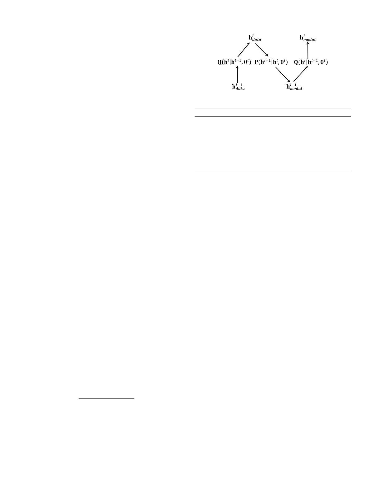
Fig. 3: Training the lth RBM by CD algorithm.
Algorithm 1. Pre-training a DBN in a layer-wise manner
Input: Training data h
0
= x; initialize θ
l
= (W
l
, b
l
, c
l
) = 0,
l = 1, 2, . . . , N; learning rate ;.
Output: A DBN with N layers.
1: for l = 1 to N do
2: train the lth RBM with data h
l−1
by CD method (see Fig. 3);
3: get the well-learned parameters W
l
, b
l
and c
l
;
4: sample h
l
∼ Q(h
l
|h
l−1
; θ
l
) = P (h
l
|h
l−1
; θ
l
) by Eq. (2);
5: end for
It is difficult to perform Gibbs sampling by the conditional
distributions P (·) in Eq. (2) since they could not be factorized.
Therefore, we usually use the approximate posteriors denoted
by Q(·) for model inference and sampling, i.e., the distribution
of the lth RBM is represented by Q(h
l−1
, h
l
) during the
pre-training phase and Q(h
l
|h
l−1
) is employed to perform a
bottom-up inference. We should notice that only the posterior
Q(h
N
|h
N−1
) is identical to the true probability P (h
N
|h
N−1
)
for the top RBM while the rest of Q(·) are all approximations.
B. Learning Deep Belief Nets
Training a DBN usually falls into two learning stages: the
pre-training in a layer-wise manner and fine-tuning as a whole.
In the phase of pre-training, the bottom RBM is trained by
the original data x, then the values h
l−1
produced by the
hidden units of the (l − 1)th RBM are used to train the lth
RBM in upper layer (l = 1, 2, . . . , N). The procedure will be
repeated to train several RBMs successively and finally result
in a deep model, which is illustrated in Algorithm 1 [8]. The
deep structure can be either trained into a generative model or
a discriminative one depending on the type of RBM (with or
without label units) chosen in the top layer of a DBN.
1) Generative Model + Supervised Fine-tuning Algorith-
m: This learning procedure [1] uses a generative RBM on
the top the same as RBMs used in the lower layers when
performing layer-wise pre-training. The resulting DBN is a
generative model which provides an efficient way of realizing
approximate inference since it only requires one single bottom-
up pass to infer the values of the top-level hidden variables.
After layer-wise training in the first phase, the resulting
DBN with an extra layer representing the label units added
to the top RBM can be fine-tuned by BP or SGD algorithms.
Then it is capable of performing classification and recognition.
We might also explain it, in another way, that the pre-trained
parameters of DBN are employed to initialize a multilayer
neural network which is then trained in a traditional gradient-
based manner.
Authorized licensed use limited to: SOUTH CHINA UNIVERSITY OF TECHNOLOGY. Downloaded on March 28,2020 at 14:23:28 UTC from IEEE Xplore. Restrictions apply.


