6
0.0
0.5
1.0
F
1
-score
5 10
Bayes factor comparison
950
1000
1050
1100
R
i
(a)
5 10 15
Generation
(b)
10% 25%
Model space
0.0
0.5
1.0
F
1
(c)
10% 25%
{
ˆ
H
i
}
25% 75%
{
ˆ
H
0
}
ˆ
σ
x
i,2
ˆ
σ
y
i,2
ˆ
σ
z
i,2
ˆ
σ
x
i,3
ˆ
σ
y
i,3
ˆ
σ
z
i,3
ˆ
σ
x
i,4
ˆ
σ
y
i,4
ˆ
σ
z
i,4
Coupling qubit/axis
1
2
3
Qubit, i
(d)
∈ T
0
/∈ T
0 /∈ T
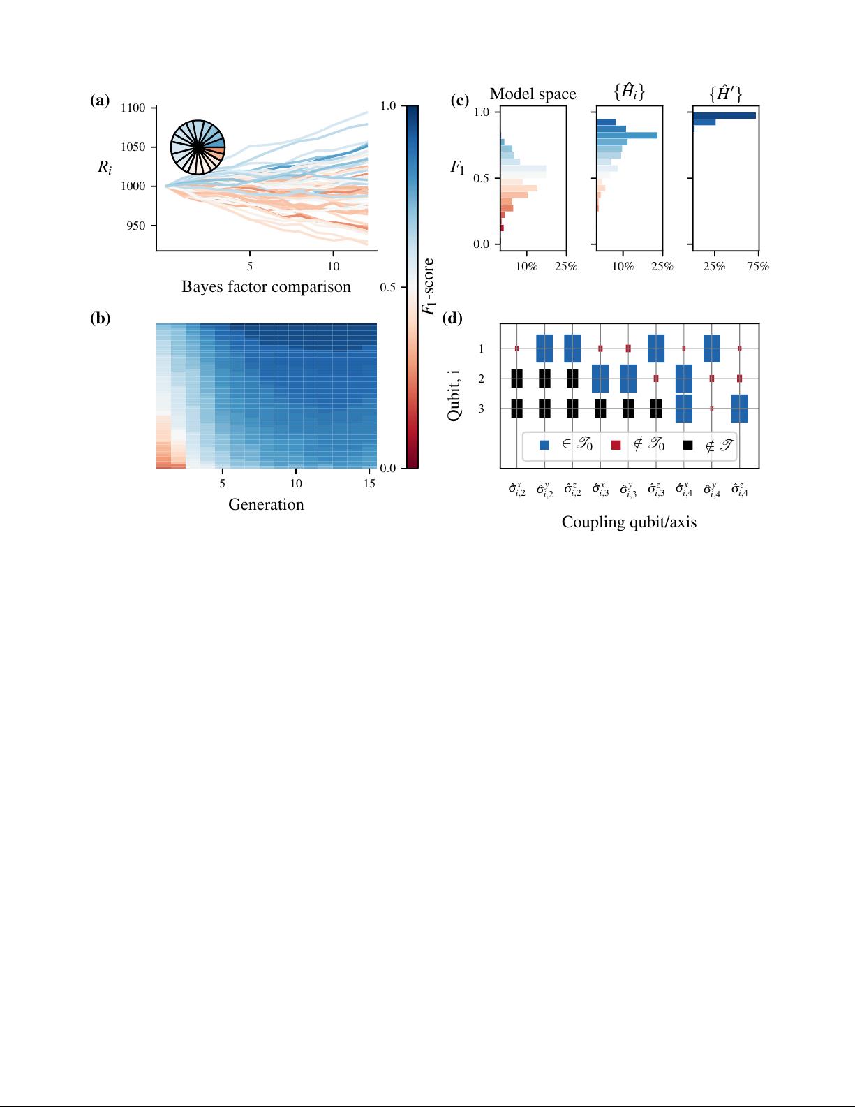
FIG. 4. Genetic algorithm exploration strategy within QMLA. (a-b), Single instance of QMLA. The genetic algorithm
runs for N
g
= 15 generations, where each generation tests N
m
= 60 models. (a), Ratings of all models in a single genetic
algorithm generation. Each line represents a unique model and is coloured by the F
1
-score of that model. Inset, the selection
probabilities resulting from the final ratings of this generation, i.e. the models’ chances of being chosen as a parent to a
new model. Only a fraction of models are assigned selection probability, while the remaining poorer-performing models are
truncated. (b), Gene pool progression for N
m
= 60, N
g
= 15. Each tile at each generation represents a model by its F
1
-score.
(c-d), Results of 100 QMLA instances using the genetic algorithm exploration strategy. (c), The model space in
which QMLA searches. (Left) The total model space contains 2
18
≈ 250, 000 candidate models; normally distributed around
¯
f = 0.5 ± 0.14. (Centre), The models explored during the model search of all instances combined, {
ˆ
H
i
}, show that QMLA
tends towards stronger models overall, with models considered having
¯
f = 0.76 ± 0.15 from ∼ 43, 000 chromosomes across the
instances, i.e. each instance trains ∼ 430 distinct models. (Right), Champion models from each instance, showing QMLA finds
strong models in general, and in particular finds the true model
ˆ
H
0
(with f = 1) in 72% of cases, and f ≥ 0.88 in all instances.
(d), Hinton diagram showing the rate at which each term is found within the winning model,
ˆ
H
0
. The size of the blocks show
the frequency with which they are found, while the colour indicates whether that term was in the true model (blue) or not
(red). Terms represent the coupling between two qubits, e.g ˆσ
x
(1,3)
couples the first and third qubits along the x-axis. We test
four qubits with full connectivity, resulting in 18 unique terms (terms with black rectangles are not considered by the GA).
• pairs of models connected by an edge, (
ˆ
H
i
,
ˆ
H
j
), are
compared through BF, giving B
ij
;
• the model indicated as inferior by B
ij
transfers
some of its rating to the superior model: the quan-
tity transferred, ∆R
ij
, reflects
– the statistical evidence given by B
ij
;
– the initial ratings of both models, {R
i
, R
j
}.
The ratings of models on µ therefore increase or de-
crease depending on their relative performance, shown
for an exemplary generation in Fig. 4a.
We use a roulette selection for the design of new candi-
date models: two models are selected from µ to become
parents and spawn offspring. The selection probability
for each model
ˆ
H
i
∈ µ is proportional to R
i
after all
comparisons on µ; the strongest
N
m
/3 models on µ are
available for selection as parents while evidently weaker
models are discarded, see Fig. 4(a - inset). This proce-
dure is repeated until N
m
models are proposed; these do
not have to be new – QMLA may have considered any
given model previously – but all models within a gen-
eration should be distinct. We show the progression of


