Published as a conference paper at ICLR 2020
Depth
Correction
Corrected Pseudo-LiDAR Point CloudSparse LiDAR Point Cloud
Dense Pseudo-LiDAR Point Cloud
KNN
graph
Weight Sharing
Feature
Extractor
left
feature
map
right
feature
map
3D conv
softmax
Disparity
Cost
Volume
Convert
Depth
Cost
Volume
Dense Predicted Depth Map
Feature
Extractor
Left Image
<latexit sha1_base64="ac35sPpnobXhLFI3vIXtMm+1InU=">AAAB6nicbVDLSgNBEOzxGRMfMR69DEYhp7AbD3qSgBe9RTQPSJYwO5lNhszOLjOzQljiF+jFgxK8+kXe/Bsnj4MmFjQUVd10d/mx4No4zjdaW9/Y3NrO7GRzu3v7B/nDQkNHiaKsTiMRqZZPNBNcsrrhRrBWrBgJfcGa/vB66jcfmdI8kg9mFDMvJH3JA06JsdL9bVd080Wn7MyAV4m7IMVqYfL8VDrN1br5r04voknIpKGCaN12ndh4KVGGU8HG2U6iWUzokPRZ21JJQqa9dHbqGJ9ZpYeDSNmSBs/U3xMpCbUehb7tDIkZ6GVvKv7ntRMTXHopl3FimKTzRUEisInw9G/c44pRI0aWEKq4vRXTAVGEGptO1obgLr+8ShqVsntertzZNK5gjgwcwwmUwIULqMIN1KAOFPrwAm/wjgR6RRP0MW9dQ4uZI/gD9PkDNQyP9A==</latexit>
<latexit sha1_base64="emBOe26klE0Zw/kQRczFLd//sRU=">AAAB6nicbVDLSgNBEOzxGRMfMR69DEYhp7AbD3qSgBe9RTQPSJYwO5lNhszOLjOzQljiF+jFgxK8+kXe/Bsnj4MmFjQUVd10d/mx4No4zjdaW9/Y3NrO7GRzu3v7B/nDQkNHiaKsTiMRqZZPNBNcsrrhRrBWrBgJfcGa/vB66jcfmdI8kg9mFDMvJH3JA06JsdL9bVd180Wn7MyAV4m7IMVqYfL8VDrN1br5r04voknIpKGCaN12ndh4KVGGU8HG2U6iWUzokPRZ21JJQqa9dHbqGJ9ZpYeDSNmSBs/U3xMpCbUehb7tDIkZ6GVvKv7ntRMTXHopl3FimKTzRUEisInw9G/c44pRI0aWEKq4vRXTAVGEGptO1obgLr+8ShqVsntertzZNK5gjgwcwwmUwIULqMIN1KAOFPrwAm/wjgR6RRP0MW9dQ4uZI/gD9PkDPiSP+g==</latexit>
<latexit sha1_base64="Nd9wGqAnyDkpEBh0VAa7gM/R0VQ=">AAAB6nicbVDLTgJBEOzFF4IPxKOXiWjCieziQU+GxItHjPJIYENmh1mYMDuzmZk1IRv8Ar140BCvfpE3/8bhcVCwkk4qVd3p7gpizrRx3W8ns7G5tb2T3c3l9/YPDgtHxaaWiSK0QSSXqh1gTTkTtGGY4bQdK4qjgNNWMLqZ+a1HqjST4sGMY+pHeCBYyAg2Vrof9nivUHIr7hxonXhLUqoVp89P5bN8vVf46vYlSSIqDOFY647nxsZPsTKMcDrJdRNNY0xGeEA7lgocUe2n81Mn6NwqfRRKZUsYNFd/T6Q40nocBbYzwmaoV72Z+J/XSUx45adMxImhgiwWhQlHRqLZ36jPFCWGjy3BRDF7KyJDrDAxNp2cDcFbfXmdNKsV76JSvbNpXMMCWTiBUyiDB5dQg1uoQwMIDOAF3uDd4c6rM3U+Fq0ZZzlzDH/gfP4AZEaQEw==</latexit>
<latexit sha1_base64="+h3HGUomtKmMBqcbNGjX0uzF+Hk=">AAAB6nicbVDLTgJBEOzFF4IPxKOXiWjCieziQU+GxItHjPJIYENmh1mYMDuzmZk1IRv8Ar140BCvfpE3/8bhcVCwkk4qVd3p7gpizrRx3W8ns7G5tb2T3c3l9/YPDgtHxaaWiSK0QSSXqh1gTTkTtGGY4bQdK4qjgNNWMLqZ+a1HqjST4sGMY+pHeCBYyAg2Vrof9lSvUHIr7hxonXhLUqoVp89P5bN8vVf46vYlSSIqDOFY647nxsZPsTKMcDrJdRNNY0xGeEA7lgocUe2n81Mn6NwqfRRKZUsYNFd/T6Q40nocBbYzwmaoV72Z+J/XSUx45adMxImhgiwWhQlHRqLZ36jPFCWGjy3BRDF7KyJDrDAxNp2cDcFbfXmdNKsV76JSvbNpXMMCWTiBUyiDB5dQg1uoQwMIDOAF3uDd4c6rM3U+Fq0ZZzlzDH/gfP4AbV6QGQ==</latexit>
<latexit sha1_base64="0UTOjvAXMEJksx/hVAkO9/WjhJo=">AAAB9HicbVA7SwNBEN7zGeMrammzGgSrcBcLrSSQxjKCeUByhL29SbJk7+HuXDQcKaytxcZCEVt/jJ3/xs2j0MQPBj6+b4aZ+bxYCo22/W0tLa+srq1nNrKbW9s7u7m9/ZqOEsWhyiMZqYbHNEgRQhUFSmjECljgSah7/fLYrw9AaRGFNziMwQ1YNxQdwRkayS23Wwj3mPpCx6N2Lm8X7AnoInFmJF86upOP5aeHSjv31fIjngQQIpdM66Zjx+imTKHgEkbZVqIhZrzPutA0NGQBaDedHD2iJ0bxaSdSpkKkE/X3RMoCrYeBZzoDhj09743F/7xmgp0LNxVhnCCEfLqok0iKER0nQH2hgKMcGsK4EuZWyntMMY4mp6wJwZl/eZHUigXnrFC8Nmlckiky5JAck1PikHNSIlekQqqEk1vyTF7JmzWwXqx362PaumTNZg7IH1ifP32HlYs=</latexit>
<latexit sha1_base64="GkKr4lOisyHRnKH92XrPamM93Wk=">AAAB9XicbVA9SwNBEN3zM8avqKXNaRCswl0stJJAGssI5gOSM+ztTZIle3vH7pwxHCmsrQUbC0Vs/S92/hs3H4UmPhh4vDfDzDw/Flyj43xbS8srq2vrmY3s5tb2zm5ub7+mo0QxqLJIRKrhUw2CS6giRwGNWAENfQF1v18e+/U7UJpH8gaHMXgh7Ure4YyikW7L7RbCPaYBxNgbtXN5p+BMYC8Sd0bypaOBeCw/PVTaua9WELEkBIlMUK2brhOjl1KFnAkYZVuJhpiyPu1C01BJQ9BeOrl6ZJ8YJbA7kTIl0Z6ovydSGmo9DH3TGVLs6XlvLP7nNRPsXHgpl3GCINl0UScRNkb2OAI74AoYiqEhlClubrVZjyrK0ASVNSG48y8vklqx4J4VitcmjUsyRYYckmNySlxyTkrkilRIlTCiyDN5JW/WwHqx3q2PaeuSNZs5IH9gff4AQOuV+g==</latexit>
<latexit sha1_base64="Os4sBqyRMZjol0WZQqJOURH20t0=">AAAB6HicdVDLSgNBEJyNrxhfUY9eBoPgadmNhyQnA3rwmIB5YLKE2UknGTM7u8zMCmHJF3jxoEg8+jdevfk3ziYKPgsaiqpuurr9iDOlHefNyiwtr6yuZddzG5tb2zv53b2mCmNJoUFDHsq2TxRwJqChmebQjiSQwOfQ8sdnqd+6AalYKC71JAIvIEPBBowSbaT6VS9fcOzKScUtl/Bv4trOHIXTl1mKp1ov/9rthzQOQGjKiVId14m0lxCpGeUwzXVjBRGhYzKEjqGCBKC8ZB50io+M0seDUJoSGs/VrxMJCZSaBL7pDIgeqZ9eKv7ldWI9KHsJE1GsQdDFokHMsQ5xejXuMwlU84khhEpmsmI6IpJQbX6TM0/4vBT/T5pF2z2xi3WnUD1HC2TRATpEx8hFJVRFF6iGGogiQLfoHj1Y19ad9WjNFq0Z62NmH32D9fwOka2R7g==</latexit>
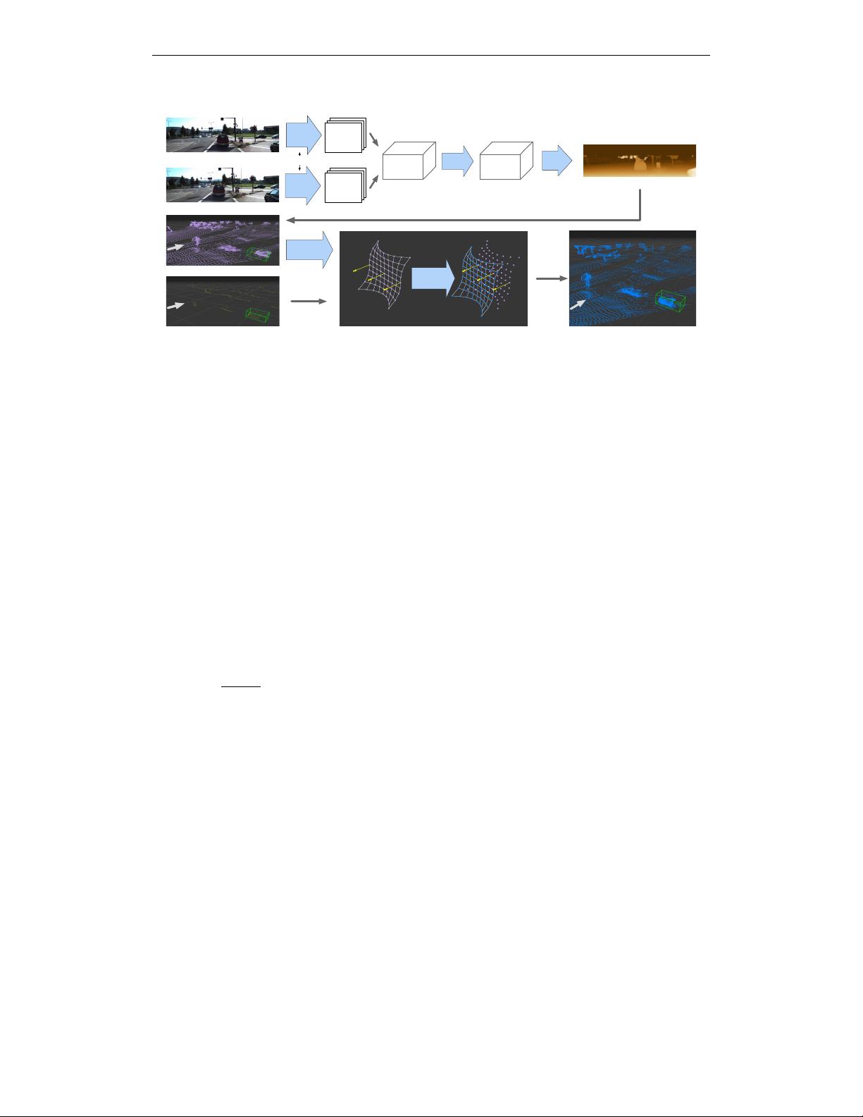
Figure 5:
The whole pipeline of improved stereo depth estimation:
(top) the stereo depth network (SDN)
constructs a depth cost volume from left-right images and is optimized for direct depth estimation; (bottom) the
graph-based depth correction algorithm (GDC) refines the depth map by leveraging sparser LiDAR signal. The
gray arrows indicates the observer’s view point. We superimpose the (green) ground-truth 3D box of a car, the
same one in Figure 1. The corrected points (blue; bottom right) are perfectly located inside the ground truth box.
throughout — which is clearly violated by the reciprocal depth to disparity relation (Figure 2). For
example, it may be completely appropriate to locally smooth two neighboring pixels with disparity
85 and 86 (changing the depth by a few cm to smooth out a surface), whereas applying the same
kernel for two pixels with disparity 5 and 6 could easily move the 3D points by 10m or more.
Taking this insight and the central assumption of convolutions — all neighborhoods can be operated
upon in an identical manner — into account, we propose to instead construct the depth cost volume
C
depth
, in which
C
depth
(u, v, z, :)
will encode features describing how likely the depth
Z(u, v)
of
pixel
(u, v)
is
z
. The subsequent 3D convolutions will then operate on the grid of depth, rather than
disparity, affecting neighboring depths identically, independent of their location. The resulting 3D
tensor S
depth
is then used to predict the pixel depth similar to Equation 3
Z(u, v) =
X
z
softmax(−S
depth
(u, v, z)) × z.
We construct the new depth volume,
C
depth
, based on the intuition that
C
depth
(u, v, z, :)
and
C
disp
u, v,
f
U
× b
z
, :
should lead to equivalent “cost”. To this end, we apply a bilinear interpolation
to construct
C
depth
from
C
disp
using the depth-to-disparity transform in Equation 2. Specifically, we
consider disparity in the range of
[0, 191]
following PSMNet (Chang & Chen, 2018), and consider
depth in the range of
[1m, 80m]
and set the grid of depth in
C
depth
to be 1m. Figure 5 (top) depicts
our stereo depth network (SDN) pipeline. Crucially, all convolution operations are operated on
C
depth
exclusively. Figure 4 compares the median values of absolute depth estimation errors using
the disparity cost volume (i.e., PSMNet) and the depth cost volume (SDN) (see subsection D.5 for
detailed numbers). As expected, for faraway depth, SDN leads to drastically smaller errors with only
marginal increases in the very near range (which disparity based methods over-optimize). See the
appendix for the detailed setup and more discussions.
4 DEPTH CORRECTION
Our SDN significantly improves depth estimation and more precisely renders the object contours
(see Figure 3). However, there is a fundamental limitation in stereo because of the discrete nature of
pixels: the disparity, being the difference in the horizontal coordinate between corresponding pixels,
has to be quantized at the level of individual pixels while the depth is continuous. Although the
quantization error can be alleviated with higher resolution images, the computational depth prediction
cost scales cubically with resolution— pushing the limits of GPUs in autonomous vehicles.
We therefore explore a hybrid approach by leveraging a cheap LiDAR with extremely sparse (e.g.,
4 beams) but accurate depth measurements to correct this bias. We note that such sensors are too
5


