使用ATLAS探测器在13 TeV pp碰撞中搜索低质量Dijet共振

48 浏览量更新于2024-07-16 收藏 703KB PDF 举报

"这篇公开访问的文章是ATLAS合作团队发表的关于在13 TeV质心能量的pp碰撞中利用ATLAS探测器进行低质量双喷流共振搜索的研究。研究中，他们面对的一个主要挑战是单射流触发器在低横向动量下的数据采集速率远低于标准模型多喷流产生的速率，这限制了亚TeV质量共振的搜索效率。为解决这个问题，研究者采用了一种新的方法，即只记录由射流触发算法计算出的事件信息，这样能在降低存储需求的同时提高事件发生率。他们的目标是寻找450到1800 GeV质量范围内的双喷流共振现象。分析的数据集最高集成照度达到29.3 fb-1。经过分析，没有发现任何异常现象，因此，他们对新粒子引起的双喷流质量分布的高斯形贡献以及与夸克有轴向矢量耦合的暗物质粒子模型设定了限制。" 这篇论文详细介绍了在大型强子对撞机(Large Hadron Collider, LHC)上，使用ATLAS实验装置进行的一次低质量双喷流共振搜索。在13 TeV的质心能量下，由于单个射流触发器在低横动量区域的数据采集能力有限，搜索可能受到统计上的限制。为了突破这个限制，研究者设计了一种创新的方法，即只保存由触发器计算的事件信息，而不是完整的事件记录，从而在保持较高事件处理速度的同时减少存储需求。研究的焦点在于450到1800 GeV质量区间内的双喷流共振，这是一个可能揭示新物理现象的领域。在这个范围内，他们分析了高达29.3 fb-1的综合照度数据，这些数据是在13 TeV的碰撞能级下收集的。通过对数据的深入分析，没有观察到超出标准模型预期的信号，这意味着在设定的质量范围内没有发现新的粒子。因此，他们根据分析结果，对新粒子（如可能存在的超对称粒子）导致的双喷流质量分布的高斯形贡献设定了上限，同时也对暗物质粒子模型（特别是那些通过轴向矢量耦合与夸克相互作用的模型）给出了限制。这项工作的结果不仅提供了对现有理论模型的检验，还展示了在处理大量数据时如何优化触发和存储策略，以提高对新物理现象的敏感性。同时，它也为未来类似的低能标搜索提供了方法论上的参考。

beyond the range, to 2970 (3490) GeV for the jy



j < 0.6

(0.3) signal selection, and the fit is evaluated at the center of

the window.

In each sliding window, three functional forms are fit to

the data: a five-parameter function of the form

fðxÞ¼p

ð1 − xÞ

þp

ln xþp

ln x

; ð1Þ

where p

are free parameters and x ≡ m

ﬃﬃﬃ

; a four-

parameter function, which is the same as Eq. (1) but with

¼ 0; and a four-parameter function used by the UA2

Collaboration [28], defined as

fðxÞ¼

−p

x−p

: ð2Þ

The function used for each signal selection is the one that

yields the best χ

over the full fitted m

range. An

alternative function is chosen to evaluate a systematic

uncertainty. For the signal selection with jy



j < 0.6,

Eq. (1) is used, yielding a χ

p value of 0.13, while the

alternative function is the four-parameter function with a χ

p value of 0.11. For the signal selection with jy



j < 0.3, the

four-parameter version of Eq. (1) yields the best χ

p value

of 0.42 and the alternative function is Eq. (2), with a χ

p value of 0.35.

The size of the sliding window is optimized to yield the

best χ

value for the full m

range while still being larger

than the width of the expected signals and therefore

insensitive to potential signal contributions. This latter

requirement is checked by including signal models in

pseudo-data samples and studying the dependence of the

signal sensitivity on different window sizes.

Systematic uncertainties in the estimate of the back-

ground used in setting limits include the uncertainty due to

the choice of functional form and uncertainties in the fit

parameter values. The effect of the choice of functional

form is evaluated by comparing the nominal function to the

alternative. The uncertainties in the fit parameter values are

evaluated using pseudoexperiments, where the pseudodata

are drawn from Poisson fluctuations around the nominal

background model.

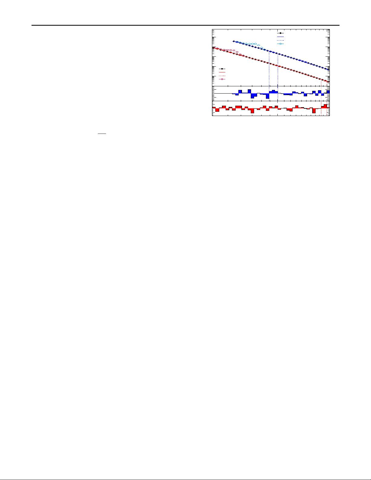
Results and limits.—Figure 4 shows the invariant mass

distributions for dijet events in each signal region including

the results from the sliding-window background estimates.

The χ

p value of the overall background is 0.13 for the



j < 0.6 signal selection and 0.42 for the jy



j < 0.3 signal

selection, indicating the data agrees well with the back-

ground estimate. The most discrepant interval identified by

the BumpHunter algorithm [33,34] is 889–1007 GeV for

events with jy



j < 0.6. Accounting for statistical uncer-

tainties only, the probability of observing a deviation at

least as significant as that observed in data, anywhere in this

distribution, is 0.44 and corresponds to significance of

0.16σ. Thus, there is no evidence of any localized excess.

Limits are set on both a leptophobic Z

simplified

dark-matter model [36] and a generic Gaussian model.

The Z

simplified model assumes axial-vector couplings to

SM quarks and to a Dirac fermion dark-matter candidate.

No interference with the SM is simulated. Signal samples

were generated so that the decay rate of the Z

into dark-

matter particles is negligible and the dijet production rate

and resonance width depend only on the coupling of the Z

to quarks, g

, and the mass of the resonance, m

[9]. The

model’s matrix elements were calculated in M

RAPH

[37] and parton showering was performed in P

YTHIA

8 [38]

with the A14 set of tuned parameters for underlying event

[39] and NNPDF2.3 parton distribution functions [40].

The width of a Z

resonance with g

¼ 0.10, including

parton shower and detector resolution effects, is approx-

imately 7%. Limits are set on the cross section, σ, times

acceptance, A, times branching ratio, B, of the model, and

then displayed in the ðg

Þ plane [41]. The acceptance

for a mass of 550 GeV is 20% for a Z

simplified model

with g

¼ 0.10 for the jy



j < 0.3 signal selection, and 41%

for a signal of mass equal to 750 GeV for the jy



j < 0.6

signal selection.

Limits are also set on a generic model where the signal is

modeled as a Gaussian contribution to the observed m

distribution. For a given mean mass, m

, four different

Gaussian widths are considered: a width equal to the

simulated mass resolution (which ranges between 4%

and 6%), and the fixed fractions 5%, 7%, and 10% of

. As the width increases, the expected signal contribu-

tion is distributed across more bins. Wider signals are

Events / Bin

[GeV]m

500 600 700 800 900

1000

2−

[GeV]

500 600 700 800 900

1000

2000

2−

Significance

ATLAS

, |y*| < 0.3

-1

Data, 3.6 fb

Background fit

BumpHunter interval

x 500σZ’,

= 0.1

= 550 GeV, g

Z’

, |y*| < 0.6

-1

Data, 29.3 fb

Background fit

BumpHunter interval

x 500σZ’,

= 0.1

= 750 GeV, g

Z’

value = 0.6pBH

value = 0.42p

value = 0.44pBH

value = 0.13p

FIG. 4. The reconstructed dijet mass distribution (filled points)

for events in the jy



j < 0 . 3 and jy



j < 0 . 6 signal regions. Solid

lines depict the background estim ate obtained by a sliding-

window fit. Overall agreement between the background estimate

and the data is quantified by the χ

p value. The most discrepant

localized excess in either signal region identified by the Bump-

Hunter algorithm is indicated by the vertical lines. The open

points show two possible signal models. The lower panels show

the bin-by-bin significances of differences between the data and

the background estimate, considering only statistical uncertain-

ties (see Ref. [35]).

PHYSICAL REVIEW LETTERS 121, 081801 (2018)

081801-4

剩余19页未读，继续阅读

weixin_38690095

粉丝: 4
资源: 914

使用ATLAS探测器在13 TeV pp碰撞中搜索低质量Dijet共振

在大型强子对撞机上使用ATLAS探测器测量的s = 13 TeV pp相互作用中的带电粒子分布

搜索新的共振，在事件中有一个轻子和缺少横向动量的pp碰撞中的s = 13 TeV的pp碰撞与ATLAS探测器

使用ATLAS探测器在s = 13 TeV pp碰撞中具有两个强子τ轻子的事件中搜索直接的stau产生

使用ATLAS探测器在s = 13 TeV的pp碰撞中搜索衰减至τν的高质量共振

使用ATLAS探测器在LHC的s = 13 TeV pp碰撞中包含两个光子和缺失的横向动量的最终状态中搜索超对称

搜索通过矢量-玻色子融合产生的希格斯玻色子，并与ATLAS探测器在s = 13 TeV pp碰撞中衰减成底夸克对

在ATLAS内部探测器和μ子光谱仪中搜索在s = 13 TeV pp碰撞中pp碰撞中产生的长寿命中性粒子，这些粒子衰减成置换的强子束。

用ATLAS探测器在s = 13TeV pp碰撞中用tau轻子搜索最终状态下的charginos和中性蛋白直接产生

使用ATLAS探测器在s = 13 TeV时以pp碰撞测量pp液滴的软滴喷射质量

使用ATLAS探测器在s $$ \ sqrt {s} $$ = 13 TeV pp碰撞中搜索第三代标量幼体夸克

最新资源