Algorithm 1 Weakly-Supervised EM (fixed bias version)
Input: Initial CNN parameters θ
0
, potential parameters b
l
,
l ∈ {0, . . . , L}, image x, image-level label set z.
E-Step: For each image position m
1:
ˆ
f
m
(l) = f
m
(l|x; θ
0
) + b
l
, if z
l
= 1
2:
ˆ
f
m
(l) = f
m
(l|x; θ
0
), if z
l
= 0
3: ˆy
m
= argmax
l
ˆ
f
m
(l)
M-Step:
4: Q(θ; θ
0
) = log P (
ˆ
y|x, θ) =
P
M
m=1
log P (ˆy
m
|x, θ)
5: Compute ∇
θ
Q(θ; θ
0
) and use SGD to update θ
0
.
have the following probabilistic graphical model:
P (x, y, z; θ) = P (x)
M
Y
m=1
P (y
m
|x; θ)
!
P (z|y) . (3)
We pursue an EM-approach in order to learn the model
parameters θ from training data. If we ignore terms that do
not depend on θ, the expected complete-data log-likelihood
given the previous parameter estimate θ
0
is
Q(θ; θ
0
) =
X
y
P (y|x, z; θ
0
) log P (y|x; θ) ≈ log P (
ˆ
y|x; θ) ,
(4)
where we adopt a hard-EM approximation, estimating in the
E-step of the algorithm the latent segmentation by
ˆ
y = argmax
y
P (y|x; θ
0
)P (z|y) (5)
= argmax
y
log P (y|x; θ
0
) + log P (z|y) (6)
= argmax
y
M
X
m=1
f
m
(y
m
|x; θ
0
) + log P (z|y)
!
.(7)
In the M-step of the algorithm, we optimize Q(θ; θ
0
) ≈
log P (
ˆ
y|x; θ) by mini-batch SGD similarly to (1), treating
ˆ
y as ground truth segmentation.
To completely identify the E-step (7), we need to specify
the observation model P (z|y). We have experimented with
two variants, EM-Fixed and EM-Adapt.
EM-Fixed In this variant, we assume that log P (z|y) fac-
torizes over pixel positions as
log P (z|y) =
M
X
m=1
φ(y
m
, z) + (const) , (8)
allowing us to estimate the E-step segmentation at each
pixel separately
ˆy
m
= argmax
y
m
ˆ
f
m
(y
m
)
.
= f
m
(y
m
|x; θ
0
) + φ(y
m
, z) . (9)
Image
Image annotations
Score maps
Weakly-Supervised E-step
FG/BG
Bias
argmax
1. Cat
2. Person
3. Plant
4. Sofa
Deep Convolutional
Neural Network
Loss
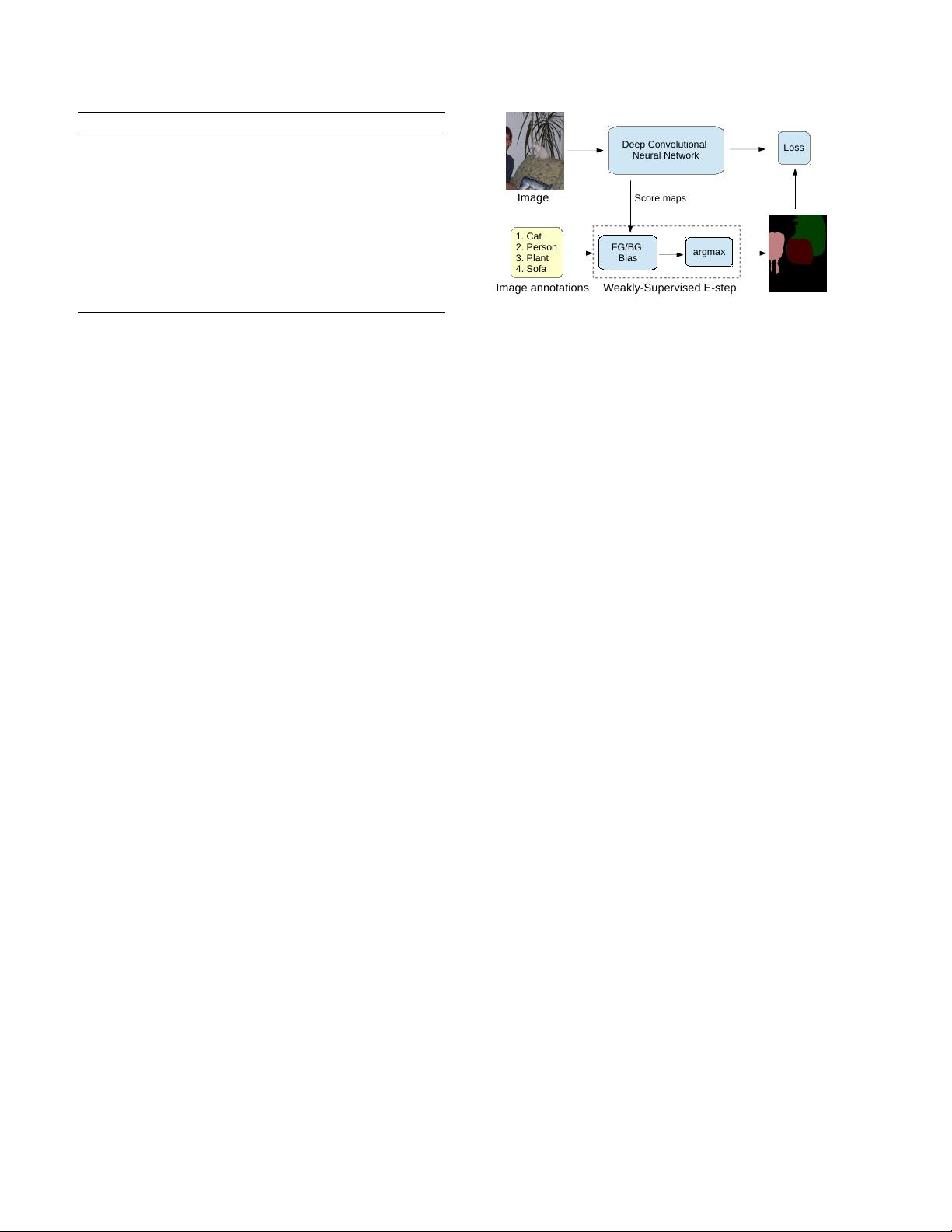
Figure 2. DeepLab model training using image-level labels.
We assume that
φ(y
m
= l, z) =
b
l
if z
l
= 1
0 if z
l
= 0
(10)
We set the parameters b
l
= b
fg
, if l > 0 and b
0
= b
bg
,
with b
fg
> b
bg
> 0. Intuitively, this potential encourages a
pixel to be assigned to one of the image-level labels z. We
choose b
fg
> b
bg
, boosting present foreground classes more
than the background, to encourage full object coverage and
avoid a degenerate solution of all pixels being assigned to
background. The procedure is summarized in Algorithm 1
and illustrated in Fig. 2.
EM-Adapt In this method, we assume that log P (z|y) =
φ(y, z) + (const), where φ(y, z) takes the form of a cardi-
nality potential [23, 33, 36]. In particular, we encourage at
least a ρ
l
portion of the image area to be assigned to class
l, if z
l
= 1, and enforce that no pixel is assigned to class
l, if z
l
= 0. We set the parameters ρ
l
= ρ
fg
, if l > 0 and
ρ
0
= ρ
bg
. Similar constraints appear in [10, 20].
In practice, we employ a variant of Algorithm 1. We
adaptively set the image- and class-dependent biases b
l
so
as the prescribed proportion of the image area is assigned to
the background or foreground object classes. This acts as a
powerful constraint that explicitly prevents the background
score from prevailing in the whole image, also promoting
higher foreground object coverage. The detailed algorithm
is described in the supplementary material.
EM vs. MIL It is instructive to compare our EM-based
approach with two recent Multiple Instance Learning (MIL)
methods for learning semantic image segmentation models
[31, 32]. The method in [31] defines an MIL classification
objective based on the per-class spatial maximum of the lo-
cal label distributions of (2),
ˆ
P (l|x; θ)
.
= max
m
P (y
m
=
l|x; θ), and [32] adopts a softmax function. While this
approach has worked well for image classification tasks
[29, 30], it is less suited for segmentation as it does not pro-
mote full object coverage: The DCNN becomes tuned to
focus on the most distinctive object parts (e.g., human face)
instead of capturing the whole object (e.g., human body).
3


