
by DoG, and filter them by key point filtering algorithm. Next, the
RoI is generated by these key points and represented by the BoW
model. At the same time, Non-RoI are also represented by the
BoW model. Finally, The visual words of RoI and Non-RoI are con-
nected to one visual word, which is used to represent the visual
features of the whole image.
Next we will introduce the RoI-BoW model in details.
Let the i-th image in the dataset be I
i
2R
N
1
N
2
; i ¼ 1; 2; ...; N,
the original image dataset is denoted as D as follows
D ¼fI
1
; I
2
; ...; I
N
g;
where N is the amount of images, N
1
and N
2
represent the size of
images. An input image can be seen as two variable function on
the rectangle
I
i
ðx; yÞ; ðx; yÞ2½1; 2; ...; N
1
½1; 2; ...; N
2
; i ¼ 1; 2; ...; N:
2.1. Key points filtering
For each image, initial key points are detected firstly by differ-
ence-of-Gaussian (DoG) algorithm [44]. The difference-of-Gaussian
[44] with the scale
r
and constant multiplicative factor k can be
computed by
Dðx; y;
r
; kÞ¼Lðx; y; k
r
ÞLðx; y;
r
Þ; ð1Þ
in which, Lðx; y;
r
Þ is the scale space of an input image Iðx; yÞ. It can
be obtained by (seen in page 94 in [44])
Lðx; y;
r
Þ¼
1
2
pr
2
e
x
2
þy
2
2
r
2
Iðx; yÞ: ð2Þ
In practice, the size is usually chosen as
r
¼ 1:6 and the constant
multiplicative factor is chosen as k ¼
ffiffiffi
2
p
.
One sampling pixel(except for border pixels) is selected as key
point only if the value of Dðx; y;
r
; kÞ is larger than all of these
neighbors (in 3 3 region, the sampling pixel is the central one
and its eight neighbors, example, if the geometry coordinate is
ði; jÞ of sampling pixel, the 3 3 region includes night points, they
are ði 1; j 1Þ; ði 1; jÞ; ði 1; j þ 1Þ; ði; j 1Þ; ði; jÞ; ði; j þ 1Þ;
ði þ 1; j 1Þ; ði þ 1; jÞ; ði þ 1; j þ 1Þ) or smaller than all of them.
After the DoG algorithm, the set of the initial key points of
image I
i
is obtained and denoted as
P
i
¼fP
i
1
; P
i
2
; ...; P
i
S
i
g;
where S
i
is the number of key points of image I
i
.
Since initial key points are too many, a filter algorithm is used to
remove some sparse points and retain the points distributed den-
sely. An example is illustrated in Fig. 3 and the filtering algorithm
is introduced as follows.
The filtering operator is denoted as h,
h : P
i
¼ P
i
1
; P
i
2
; ...; P
i
S
i
no
! Q
i
¼ Q
i
1
; Q
i
2
; ...; Q
i
T
i
no
; ð3Þ
where T
i
is the number of key points of image I
i
after filtering.
Each initial key point is judged by a boolean function as formula
(4),
bP
i
j
¼
1; lðP
i
j
Þ P L;
0; lðP
i
j
Þ < L;
(
ð4Þ
where b ¼ 1 means retaining the point, and b ¼ 0 means removing. l
is a statistic function to calculate the number of key points around
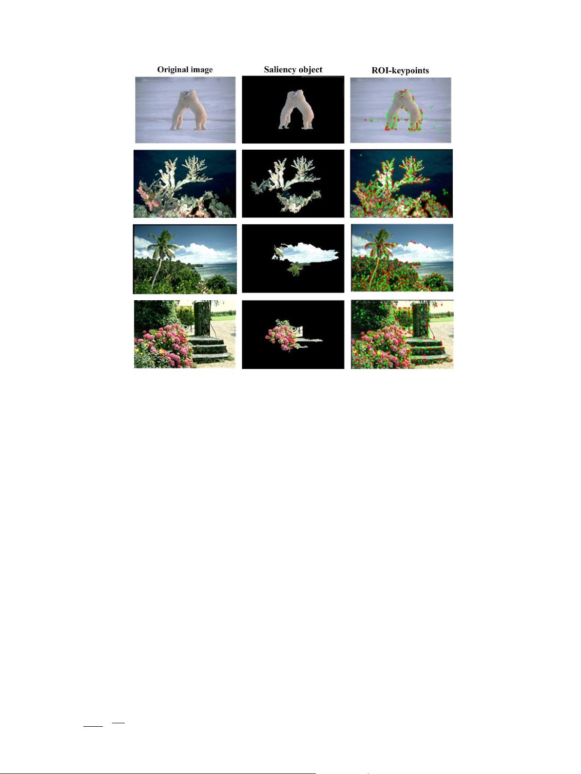
Fig. 1. The above two pictures show the similarity between salient regions detection and region of interest with difference-of-Gaussian. the below two pictures tell us that
there is significant difference. The first column is the original images. The middle column is the corresponding salient regions. The last column is region of interest with
difference-of-Gaussian (the keypoints are labeled with red points). (For interpretation of the references to colour in this figure legend, the reader is referred to the web version
of this article.)
J. Zhang et al. / J. Vis. Commun. Image R. 26 (2015) 37–49
39
剩余12页未读,继续阅读

weixin_38659789
- 粉丝: 4
- 资源: 923
 我的内容管理
展开
我的内容管理
展开


最新资源
- 最优条件下三次B样条小波边缘检测算子研究
- 深入解析:wav文件格式结构
- JIRA系统配置指南:代理与SSL设置
- 入门必备:电阻电容识别全解析
- U盘制作启动盘:详细教程解决无光驱装系统难题
- Eclipse快捷键大全:提升开发效率的必备秘籍
- C++ Primer Plus中文版:深入学习C++编程必备
- Eclipse常用快捷键汇总与操作指南
- JavaScript作用域解析与面向对象基础
- 软通动力Java笔试题解析
- 自定义标签配置与使用指南
- Android Intent深度解析:组件通信与广播机制
- 增强MyEclipse代码提示功能设置教程
- x86下VMware环境中Openwrt编译与LuCI集成指南
- S3C2440A嵌入式终端电源管理系统设计探讨
- Intel DTCP-IP技术在数字家庭中的内容保护
资源上传下载、课程学习等过程中有任何疑问或建议,欢迎提出宝贵意见哦~我们会及时处理!
点击此处反馈


