4 E. Andreassen et al.
density variables cannot become zero, and the term γ is
not required.
The density filter transforms the original densities x
e
as
follows:
˜x
e
=
1
i∈N
e
H
ei
i∈N
e
H
ei
x
i
(9)
In the following, the original densities x
e
are referred to as
the design variables. The filtered densities ˜x
e
are referred to
as the physical densities. This terminology is used to stress
the fact that the application of a density filter causes the
original densities x
e
to loose their physical meaning. One
should therefore always present the filtered density field ˜x
e
rather than the original density field x
e
as the solution to the
optimization problem (Sigmund 2007).
In the case where a density filter is applied, the sensitiv-
ities of the objective function c and the material volume V
with respect to the physical densities ˜x
e
are still given by
(5)and(6), provided that the variable x
e
is replaced with ˜x
e
.
The sensitivities with respect to the design variables x
j
are
obtained by means of the chain rule:
∂ψ
∂x
j
=
e∈N
j
∂ψ
∂ ˜x
e
∂ ˜x
e
∂x
j
=
e∈N
j
1
i∈N
e
H
ei
H
je
∂ψ
∂ ˜x
e
(10)
where the function ψ represents either the objective func-
tion c or the material volume V .
3 MATLAB implementation
In this section the 88 line MATLAB code (see Appendix)is
explained. The code is called from the MATLAB prompt by
means of the following line:
top88(nelx,nely,volfrac,penal,rmin,ft)
where nelx and nely are the number of elements in the
horizontal and vertical direction, respectively, volfrac is
the prescribed volume fraction f , penal is the penaliza-
tion power p, rmin is the filter radius r
min
(divided by
the element size), and the additional argument (compared to
the 99 line code) ft specifies whether sensitivity filtering
(ft = 1) or density filtering (ft = 2) should be used.
When sensitivity filtering is chosen, the 88 line code yields
practically
1
the same results as the 99 line code; e.g. the
1
The slight difference which can be observed between the 88-line and
the 99-line code is due to the difference in the SIMP formulation.
optimized MBB beam shown in Fig. 1 of the original paper
by Sigmund (2001) can be reproduced by means of the
following function call:
top88(60,20,0.5,3,1.5,1)
The most obvious differences between the 88 line code
and the 99 line code are the following: (1) the for loops
used to assemble the finite element matrices, to compute
the compliance, and to perform the filtering operation have
been vectorized, (2) the remaining arrays constructed by
means of a for loop are properly preallocated, (3) a maxi-
mum amount of code is moved out of the optimization loop
to ensure that it is only executed once, (4) a distinction is
made between the design variables x and the physical densi-
ties xPhys in order to facilitate the application of a density
filter, and (5) all subroutines have been integrated in the
main program.
The 88 line code consists of three parts: the finite ele-
ment analysis, the sensitivity or density filter, and the
optimization loop. These parts are discussed in detail in
Sections 3.1–3.3. Section 3.4 presents some results obtained
with the 88 line code.
3.1 Finite element analysis
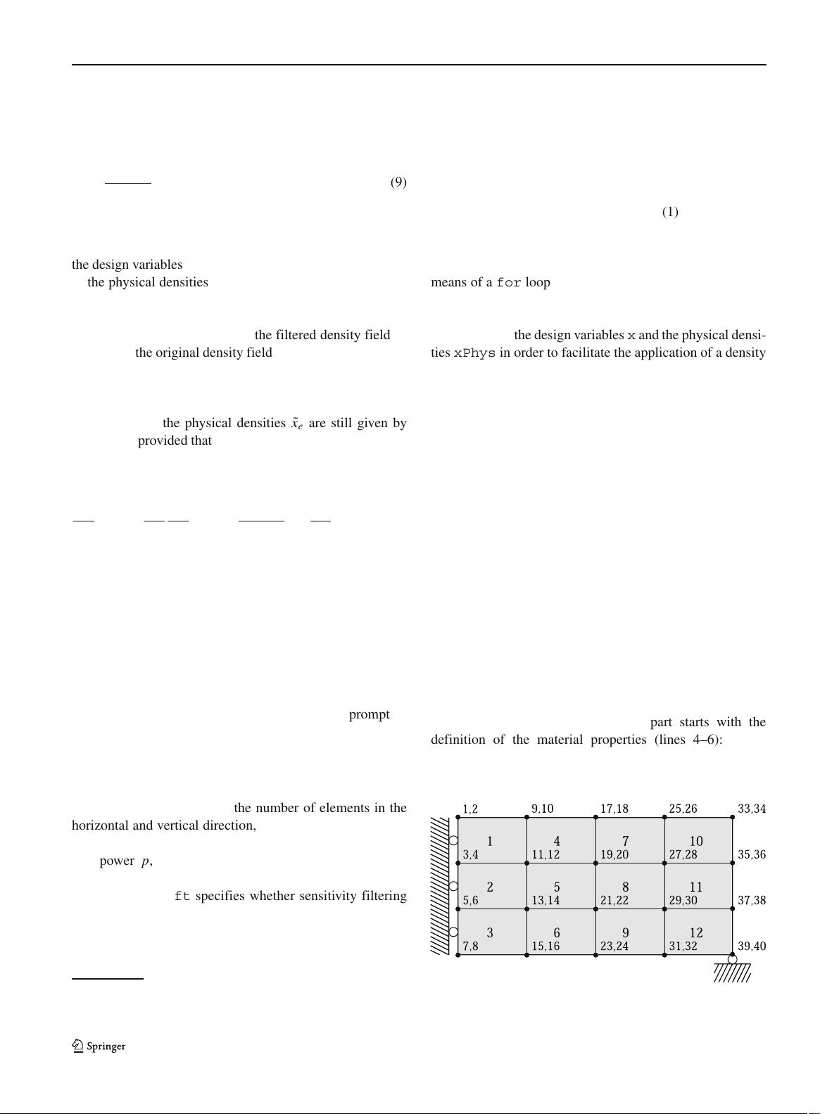
The design domain is assumed to be rectangular and dis-
cretized with square elements. A coarse example mesh
consisting of 12 elements with four nodes per element and
two degrees of freedom (DOFs) per node is presented in
Fig. 2. Both nodes and elements are numbered column-wise
from left to right, and the DOFs 2n − 1and2n corre-
spond to the horizontal and vertical displacement of node
n, respectively. This highly regular mesh can be exploited
in several ways in order to reduce the computational effort
in the optimization loop to a minimum.
The finite element preprocessing part starts with the
definition of the material properties (lines 4–6): E0 is
the Young’s modulus E
0
of the material, Emin is the
Fig. 2 The design domain with 12 elements


