R语言探索:非线性回归实战指南
需积分: 38 119 浏览量
更新于2024-07-18
3
收藏 1006KB PDF 举报
"《非线性回归分析实战:R语言指南》"
在现代数据分析领域,R语言因其丰富的统计功能和强大的图形处理能力而受到广泛赞誉。本书《Nonlinear Regression with R》由Christian Ritz和Jens Carl Streibig合著,两位作者分别来自丹麦哥本哈根大学的生命科学学院,他们在非线性回归分析方面拥有深厚的学术背景和实践经验。非线性回归是统计学中的一个重要分支,它用于研究变量之间非线性的关系,这在诸如生态学、生物学、经济学等领域有着广泛的应用。
本书的核心内容围绕如何使用R语言来执行复杂的非线性模型拟合,包括但不限于多元非线性回归、曲线拟合、混合效应模型等。作者们强调了R语言提供的统计软件包,如`nlme`(用于混合效应模型)、`ggplot2`(用于数据可视化)和`stats`(基础统计函数库)在非线性分析中的关键作用。读者将学习如何解析模型的复杂性,理解参数估计、残差分析和模型诊断,以及如何优化模型选择以提高预测准确性。
此外,书中还包含了实用案例研究,展示了如何在实际问题中应用非线性回归技术,帮助读者更好地理解和掌握R语言的使用。对于那些希望在R环境下深入探索非线性分析的读者,本书提供了丰富的资源,包括R代码示例和对R语言高级特性的介绍,使学习者能够逐步提升技能,从初级用户成长为专业分析者。
总结来说,《Nonlinear Regression with R》是一本不可多得的资源,它不仅讲解了非线性回归理论,还提供了R语言作为工具的实际操作指导,适合想要在数据分析领域进行非线性建模的研究生、研究人员以及数据分析师使用。无论是为了学术研究还是职业发展,这本书都是一个宝贵的学习资料。通过阅读和实践书中的内容,读者将能够掌握R语言在非线性回归分析中的强大功能,提升数据分析能力。
6 1 Introduction
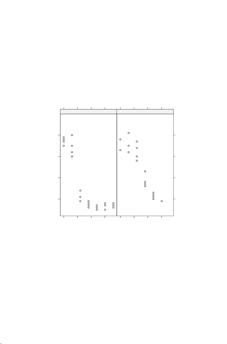
dose axis), and the parameter b is proportional to the slope at a dose equal to
e. Figure 1.3 reveals that the two curves seem to have roughly the same lower
and upper limits, and they appear to be parallel in the dose range from 20 to
100 g/ha, possibly indicating similar slopes but different inflection points.
> xyplot(DryMatter ~ Dose | Herbicide,
+ data = S.alba, scales = list(x = list(log = TRUE)),
+ ylab = "Dry matter (g/pot)",
+ xlab = "Dose (g/ha)")
Dose (g/ha)
Dry matter (g/pot)
1
2
3
4
10^1.0 10^1.5 10^2.0 10^2.5
Bentazone
10^1.0 10^1.5 10^2.0 10^2.5
Glyphosate
Fig. 1.3. The effect of increasing doses of two herbicide treatments on growth of
white mustard (Sinapis alba)plants.


剩余149页未读,继续阅读
2018-10-22 上传
2020-05-20 上传
2021-10-15 上传
2021-10-10 上传
2022-07-14 上传
2022-11-01 上传
2022-11-01 上传
2023-04-25 上传

xiaofengyulu
- 粉丝: 0
- 资源: 31
 我的内容管理
展开
我的内容管理
展开


最新资源
- Python库 | mtgpu-0.2.5-py3-none-any.whl
- endpoint-testing-afternoon:一个下午的项目,以帮助使用Postman巩固测试端点
- 经济中心
- z7-mybatis:针对mybatis框架的练习,目前主要技术栈包含springboot,mybatis,grpc,swgger2,redis,restful风格接口
- Cloudslides-Android:云幻灯同步演示应用-Android Client
- testingmk:做尼采河
- ecom-doc-static
- kindle-clippings-to-markdown:将Kindle的“剪贴”文件转换为Markdown文件,每本书一个
- 减去图像均值matlab代码-TVspecNET:深度学习的光谱总变异分解
- 自动绿色
- Alexa-Skills-DriveTime:该存储库旨在演示如何建立ALEXA技能,以帮助所有人了解当前流量中从源头到达目的地所花费的时间
- 灰色按钮克星易语言版.zip易语言项目例子源码下载
- HTML5:基本HTML5
- dubbadhar-light
- 使用Xamarin Forms创建离线移动密码管理器
- matlab对直接序列扩频和直接序列码分多址进行仿真实验源代码
