移动通信系统中的瑞利衰落信道分析

需积分: 9 42 浏览量更新于2024-09-23 收藏 152KB PDF 举报

"这篇文章来自于1997年7月的IEEE Communications Magazine，主题是‘Rayleigh Fading Channels in Mobile Digital Communication Systems’，分为第一部分：Characterization。文章探讨了在移动数字通信系统中，雷利衰落信道对通信性能的影响。" 在无线通信领域，了解和分析信道特性对于系统设计至关重要。"Rayleigh Fading Channels"是描述多径传播现象的一个关键概念，尤其在移动通信中常见。当无线电波在传播过程中遇到建筑物、树木等障碍物时，会发生反射、散射，导致信号强度在时间和空间上快速变化，形成多径衰落，即雷利衰落。描述中的"communication modulation for rayliegh fading"指出，针对这种衰落信道，需要特定的调制技术来应对。调制是通信系统中的核心环节，其目的是将信息编码到载波信号上以便传输。在雷利衰落环境中，常见的调制方式如QPSK（正交相位键控）、QAM（正交幅度调制）等可能需要配合分集技术或均衡器来增强抗衰落能力。文章提到了经典的加性高斯白噪声（AWGN）信道作为理解通信系统性能的基础。在AWGN信道中，数据样本受到统计独立的高斯噪声干扰，且无符号间干扰（ISI）。然而，实际通信系统中，接收机内的热噪声并非主要性能降级源，外部干扰，特别是具有宽频带特性的干扰，可能更为显著，这通常通过天线温度来量化。除了热噪声，信道滤波器在实际系统模型中扮演重要角色。发射端的滤波器往往用于满足法规要求，限制带宽，并可能采用预失真技术来改善非线性效应。接收端的滤波器则用于消除带外噪声，提高信噪比，并可能配合均衡器消除由信道引起的ISI。在处理雷利衰落时，多径分集技术如空间分集、时间分集和频率分集可以提高信号的可靠性。此外，先进的信道估计算法，如最小均方误差（MMSE）或最大似然（ML）估计，用于补偿信道影响，使接收端能够恢复原始信号。该文第一部分可能会深入探讨雷利衰落信道的统计特性，包括衰落的分布、深度、持续时间和相关性，以及这些特性如何影响通信系统的误码率和数据速率。接下来，可能会介绍如何通过调制、编码和分集技术来对抗这些影响，从而实现可靠通信。

IEEE Communications Magazine • July 1997

Hence, the amount of margin indicated is intended to provide

adequate received signal power for approximately 98–99 per-

cent of each type of fading variation (large- and small-scale).

A received signal, r(t), is generally described in terms of a

transmitted signal s(t) convolved with the impulse response of

the channel h

(t). Neglecting the degradation due to noise, we

write

r(t) = s(t)

(t), (2)

where * denotes convolution. In the case of mobile radios, r(t)

can be partitioned in terms of two component random vari-

ables, as follows [5]:

r(t) = m(t) x r

(t), (3)

where m(t) is called the large-scale-fading component, and

(t) is called the small-scale-fading component. m(t) is some-

times referred to as the local mean or log-normal fading

because the magnitude of m(t) is described by a log-normal

pdf (or, equivalently, the magnitude measured in decibels has

a Gaussian pdf). r

(t) is sometimes referred to as multipath or

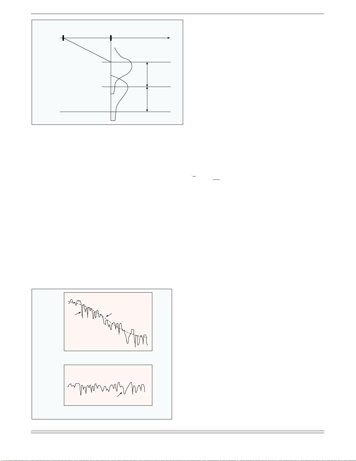
Rayleigh fading. Figure 3 illustrates the relationship between

large-scale and small-scale fading. In Fig. 3a, received signal

power r(t) versus antenna displacement (typically in units of

wavelength) is plotted, for the case of a mobile radio.

Small-scale fading superimposed on large-scale fading can

be readily identified. The typical antenna displacement

between the small-scale signal nulls is approximately a

half wavelength. In Fig. 3b, the large scale fading or local

mean, m(t), has been removed in order to view the small-

scale fading, r

(t), about some average constant power.

In the sections that follow, we enumerate some of the

details regarding the statistics and mechanisms of large-

scale and small-scale fading.

LARGE-SCALE FADING: PATH-LOSS MEAN

AND

STANDARD DEVIATION

or the mobile radio application, Okumura [6] made

some of the earlier comprehensive path-loss measure-

ments for a wide range of antenna heights and coverage

distances. Hata [7] transformed Okumura’s data into paramet-

ric formulas. For the mobile radio application, the mean path

loss,

—

(d), as a function of distance, d, between the transmit-

ter and receiver is proportional to an nth power of d relative

to a reference distance d

[3].

(4)

—

(d) is often stated in decibels, as shown below.

—

(d) (dB) = L

) (dB) + 10 n log (d/d

) (5)

The reference distance d

corresponds to a point located in

the far field of the antenna. Typically, the value of d

is taken

to be 1 km for large cells, 100 m for microcells, and 1 m for

indoor channels.

—

(d) is the average path loss (over a multi-

tude of different sites) for a given value of d. Linear regres-

sion for a minimum mean-squared estimate (MMSE) fit of

—

(d) versus d on a log-log scale (for distances greater than

) yields a straight line with a slope equal to 10n dB/decade.

The value of the exponent n depends on the frequency, anten-

na heights, and propagation environment. In free space, n = 2,

as seen in Eq. 1. In the presence of a very strong guided wave

phenomenon (like urban streets), n can be lower than 2.

When obstructions are present, n is larger. The path loss

) to the reference point at a distance d

from the trans-

mitter is typically found through field measurements or calcu-

lated using the free-space path loss given by Eq. 1. Figure 4

shows a scatter plot of path loss versus distance for measure-

ments made in several German cities [8]. Here, the path loss

has been measured relative to the free-space reference mea-

surement at d

= 100 m. Also shown are straight-line fits to

various exponent values.

The path loss versus distance expressed in Eq. 5 is an aver-

age, and therefore not adequate to describe any particular set-

ting or signal path. It is necessary to provide for variations

about the mean since the environment of different sites may

be quite different for similar transmitter-receiver separations.

Figure 4 illustrates that path-loss variations can be quite large.

Measurements have shown that for any value of d, the path

loss L

(d) is a random variable having a log-normal distribu-

tion about the mean distant-dependent value

—

(d) [9]. Thus,

path loss L

(d) can be expressed in terms of

—

(d) plus a ran-

dom variable X

, as follows [3]:

(d) (dB) = L

) (dB) + 10nlog

(d/d

) + X

(dB) (6)

where X

denotes a zero-mean Gaussian random variable (in

decibels) with standard deviation σ (also in decibels). X

site- and distance-dependent. The choice of a value for X

L d

( ) ∝













■ Figure 2. Link-budget considerations for a fading channel.

Power

transmitted

Mean

path loss

Log-normal

large-scale fading

Large-scale

fading margin

Small-scale

fading margin

Rayleigh

small-scale fading

≈ 1–2%

Base

station

Mobile

station

Distance

Power

Received

■ Figure 3. Large-scale fading and small-scale fading.

Signal

power

(dB)

(a)

Antenna

displacement

r(t)

m(t)

Signal

power

(dB)

(b)

Antenna

displacement

(t)

剩余10页未读，继续阅读

muddytu

粉丝: 0
资源: 9

移动通信系统中的瑞利衰落信道分析

最新资源