of M’s step and direction of D’s step.
Algorithm 2 AdaGraft meta-optimizer
1: Input: Optimizers M, D; initializer w
1
; > 0.
2: Initialize M, D at w
1
.
3: for t = 1, . . . , T do
4: Receive stochastic gradient g
t
at w
t
.
5: Query steps from M and D:
w
M
:= M(w
t
, g
t
), w
D
:= D(w
t
, g
t
).
6: Update with grafted step:
w
t +1
← w
t
+
kw
M
– w
t
k
kw
D
– w
t
k +
· (w
D
– w
t
) .
7: end for
Layer-wise vs. global grafting.
Two natural variants of Algorithm 2 come to mind, especially if one is
concerned about efficient implementation (see Appendix C.1). In the layer-wise version, we view w
t
as a
single parameter group (usually a tensor-shaped variable specified by the architecture), and apply AdaGraft
and its child optimizers to each group. In the global version, w
t
contains all of the model’s weights. We
discuss and evaluate both variants, but our main experimental results use layer-wise grafting.
The first experimental question addressed by AdaGraft is the following: To what degree does an optimizer’s
implicit step size schedule determine its training curve? To this end, given a set of base optimizers, we can
perform training runs for all pairs (
M
,
D
), where grafting (
A
,
A
) is understood as simply running
A
. For the
main experiments, we use SGD, Adam, and AdaGrad, all with momentum β
1
= 0.9.
All experiments were carried out on 32 cores of a TPU-v3 Pod [
JYP
+
17
], using the Lingvo [
SNW
+
19
]
sequence-to-sequence framework built on top of TensorFlow [ABC
+
16].
3.2 ImageNet classification experiments
We ran all pairs of grafted optimizers on a 50-layer residual network [
HZRS16
] with 26M parameters, trained
on ImageNet classification [
DDS
+
09
]. We used a batch size of 4096, enabled by the large-scale training
infrastructure, and a learning rate schedule consisting of a linear warmup and stepwise exponential decay. All
details can be found in Appendix C.2.
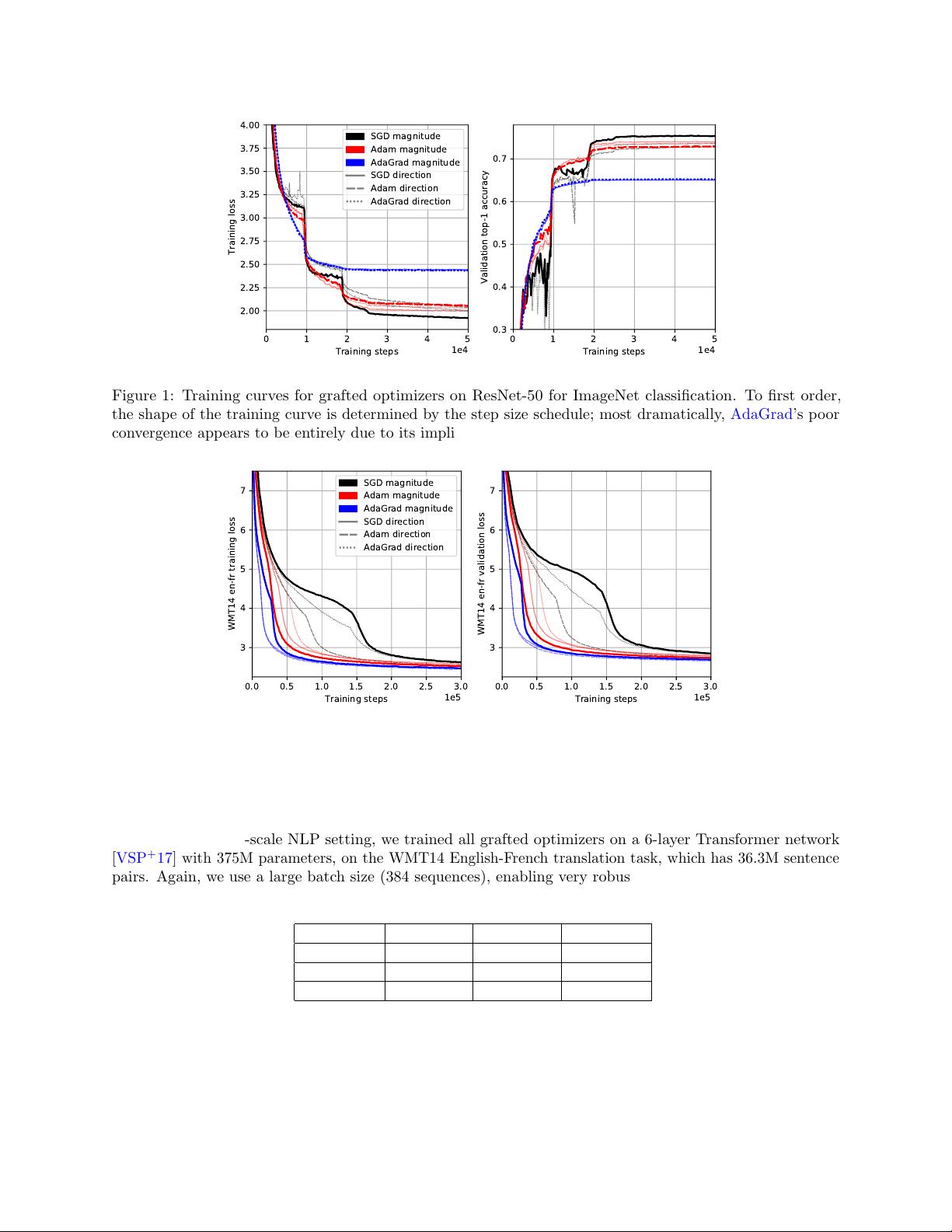
Table 2 shows top-1 and top-5 accuracies at convergence. The final accuracies at convergence, as well as
training loss curves, are very stable (
<
0.1% deviation) across runs, due to the large batch size. Figure 1
shows at a glance our main empirical observation: that the shapes of the training curves are clustered by the
choice of M, the optimizer which supplies the step magnitude.
We stress that no additional hyperparameter tuning was done in these experiments; not even the global
scalar learning rate needed adjustment. Thus, starting with N tuned optimizer setups, grafting produces a
table of N
2
setups with no additional effort. Each row of this table controls for the implicit step size schedule.
M
D SGD Adam AdaGrad
SGD 75.4 · 92.6 72.8 · 91.2 73.7 · 91.4
Adam 74.1 · 91.9 73.0 · 91.3 73.7 · 91.6
AdaGrad 65.0 · 85.9 65.1 · 86.0 65.3 · 86.3
Table 2: Top-1 and top-5 accuracies at training step t = 50K for ImageNet experiments. Averaged over 3
trials; no accuracy varied by more than 0.1%.
5


