RF采样ADC:集成数字处理的高性能数据转换器
192 浏览量
更新于2024-08-29
收藏 493KB PDF 举报
RF采样ADC(Radio Frequency Sampling Analog-to-Digital Converter)是现代数据转换器领域的一项重要进展,它在数据转换器历史上扮演了关键角色。传统上,数据转换器经历了从大型、耗能的分立元件(如DATRAC 11位50kSPS真空管ADC,功率高达500W)到高度集成的单芯片IC的转变。早期的ADC设计主要依赖于少量的数字电路,用于基本的纠错和驱动功能。
新一代的GSPS(每秒千兆样本)RF采样ADC采用65纳米CMOS技术制造,显著提高了集成度。这种技术革新使得数字处理功能得以显著增强,从而使得数据转换器从传统的模拟电路为主转变为模拟和数字电路并重的“小A大D”架构。这意味着ADC不再仅仅负责模拟信号的转换,而是能够进行复杂的数字信号处理,如滤波、校准和压缩等,提升了整体性能。
以前,ADC的设计者受限于硅工艺技术,如0.5μm、0.35μm、0.18μm到65nm的改进,使得转换速度有了显著提升。随着这些进步,RF采样ADC不仅实现了更高的采样率(GHz级别),还能够更高效地处理高速数据流,减轻FPGA(现场可编程门阵列)的数字处理负担。这为系统设计师带来了极大的灵活性,他们可以设计出通用的硬件平台,通过软件重新配置来适应不同的应用场景,节省了设计时间和成本。
此外,RF采样ADC的优势还包括功耗降低、体积减小以及噪声抑制能力增强。由于数字电路的集成,这些ADC能够在保持高性能的同时,实现更低的功耗和更紧凑的封装,这对于能源效率和小型化系统设计至关重要。
总结来说,RF采样ADC是数据转换器技术的重大飞跃,它通过集成更多数字处理功能,实现了模拟信号的高效转换和高级处理,极大地推动了电子系统设计的进步,为未来的数据采集和处理应用开辟了新的可能性。随着技术的不断发展,我们期待看到更多创新的RF采样ADC解决方案,进一步优化系统性能和效率。
RF采样采样ADC的优势的优势
数据转换器充当现实模拟世界与数字世界之间的桥梁已有数十年的历史。从占用多个机架空间并消耗大量电能
(例如DATRAC 11位50kSPS真空管ADC的功耗为500W)的分立元件起步,数据转换器现已蜕变为高度集成的
单芯片IC。从款商用数据转换器诞生以来,对更快数据速率的无止境需求驱动着数据转换器不断向前发展。
ADC的化身是采样速率达到GHz的RF采样ADC。早先的ADC设计使用的数字电路非常少,主要用于纠错和数字
驱动器。新一代GSPS(每秒千兆样本)转换器(也称为RF采样ADC)利用65 nm CMOS技术实现,可以集成许多数
字处理功能来增强ADC的性能。这样,数据转换器便从20世纪90年代中期和
数据转换器充当现实模拟世界与数字世界之间的桥梁已有数十年的历史。从占用多个机架空间并消耗大量电能(例如
DATRAC 11位50kSPS真空管ADC的功耗为500W)的分立元件起步,数据转换器现已蜕变为高度集成的单芯片IC。从款商用
数据转换器诞生以来,对更快数据速率的无止境需求驱动着数据转换器不断向前发展。ADC的化身是采样速率达到GHz的RF
采样ADC。
早先的ADC设计使用的数字电路非常少,主要用于纠错和数字驱动器。新一代GSPS(每秒千兆样本)转换器(也称为RF采
样ADC)利用65 nm CMOS技术实现,可以集成许多数字处理功能来增强ADC的性能。这样,数据转换器便从20世纪90年代中
期和21世纪早期的大A (模拟)小D (数字)式ADC变身为现在的小A大D式ADC。
这并不意味着模拟电路及其性能已衰退,而是说数字电路的数量已大幅增加,与模拟性能互为补充。这些增加的特性使得
ADC能够在ADC芯片中快速执行大量数字处理,分担FPGA的一些数字处理负荷。这就为系统设计人员开启了许多其它可能
性。现在,采用这些先进的新型GSPS ADC,系统设计人员针对各种各样的平台只需设计一种硬件,然后高效率地利用软件
重新配置该硬件,便可适应新的应用。
增强的高速数字处理增强的高速数字处理
不断缩小的CMOS工艺尺寸和先进的设计架构相结合,意味着ADC终于也能利用数字处理技术来改善性能。该突破是在
20世纪90年代早期实现的,自此之后,ADC设计人员再也没有回头。随着硅工艺的改进(从0.5 μm、0.35 μm、0.18 μm到65
nm),转换速度也得到提高。但是,几何尺寸缩小使得晶体管变小,虽然速度更快(因而带宽更高),但就模拟设计性能而言,
某些特性变得略差,例如Gm (跨导)。以前,这要通过增加更多校正逻辑来补偿。然而,那时的硅仍很昂贵,导致ADC内部的
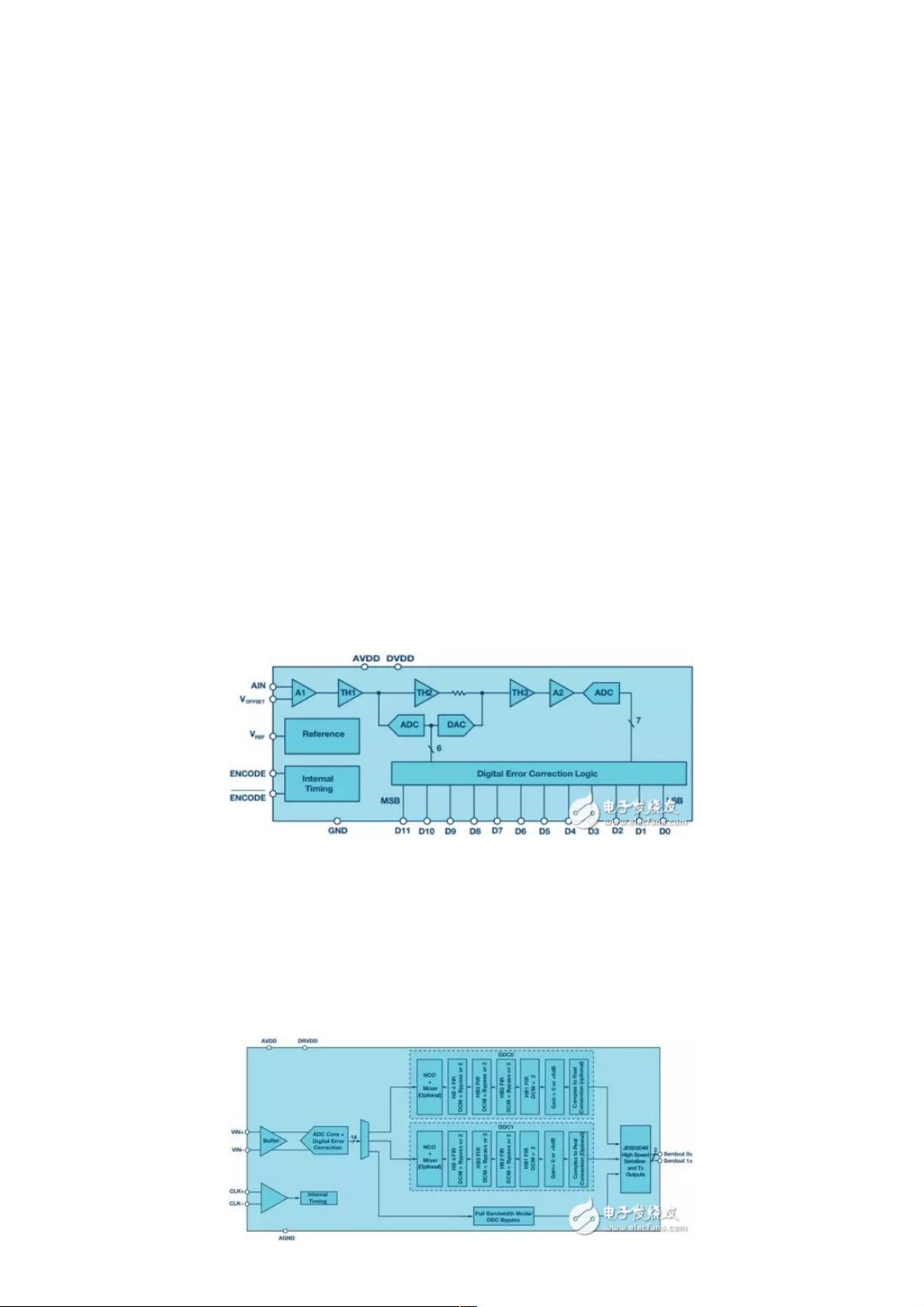
数字电路数量相对较少。图1所示为一个实例的功能框图。
图1.集成极少数字纠错逻辑的早期单芯片ADC
随着硅技术发展到深亚微米尺寸(如65 nm),数据转换器除了内核能够跑得更快(1 GSPS或更高)以外,规模经济性还使其
可以增加大量数字处理。这是再次审视后发现的一个突破性进展。通常,根据系统性能和成本要求,数字信号处理是由ASIC
或FPGA处理。ASIC是专用电路,开发需要耗费大量资金。因此,设计人员通常会让ASIC设计长期运行,以扩大ASIC开发的
投资回报。FPGA比ASIC便宜,不需要巨额开发预算。然而,由于FPGA追求支持所有应用,所以其信号处理能力会受到速度
和功效的限制。这是可以理解的,因为它具备ASIC所不具备的灵活性和重新配置能力。图2所示为一个具有可配置数字处理模
块的RF采样ADC (也称为GSPS ADC)的功能框图。
下载后可阅读完整内容,剩余6页未读,立即下载
2021-05-21 上传
2020-07-21 上传
2023-07-08 上传
2023-09-20 上传
2023-06-02 上传
2023-10-24 上传
2024-07-19 上传
2023-05-22 上传
2023-06-06 上传

weixin_38707356
- 粉丝: 17
- 资源: 958
 我的内容管理
展开
我的内容管理
展开


最新资源
- 达梦数据库DM8手册大全:安装、管理与优化指南
- Python Matplotlib库文件发布:适用于macOS的最新版本
- QPixmap小demo教程:图片处理功能实现
- YOLOv8与深度学习在玉米叶病识别中的应用笔记
- 扫码购物商城小程序源码设计与应用
- 划词小窗搜索插件:个性化搜索引擎与快速启动
- C#语言结合OpenVINO实现YOLO模型部署及同步推理
- AutoTorch最新包文件下载指南
- 小程序源码‘有调’功能实现与设计课程作品解析
- Redis 7.2.3离线安装包快速指南
- AutoTorch-0.0.2b版本安装教程与文件概述
- 蚁群算法在MATLAB上的实现与应用
- Quicker Connector: 浏览器自动化插件升级指南
- 京东白条小程序源码解析与实践
- JAVA公交搜索系统:前端到后端的完整解决方案
- C语言实现50行代码爱心电子相册教程
