Z. Zhang et al. Engineering Applications of Artificial Intelligence 67 (2018) 235–245
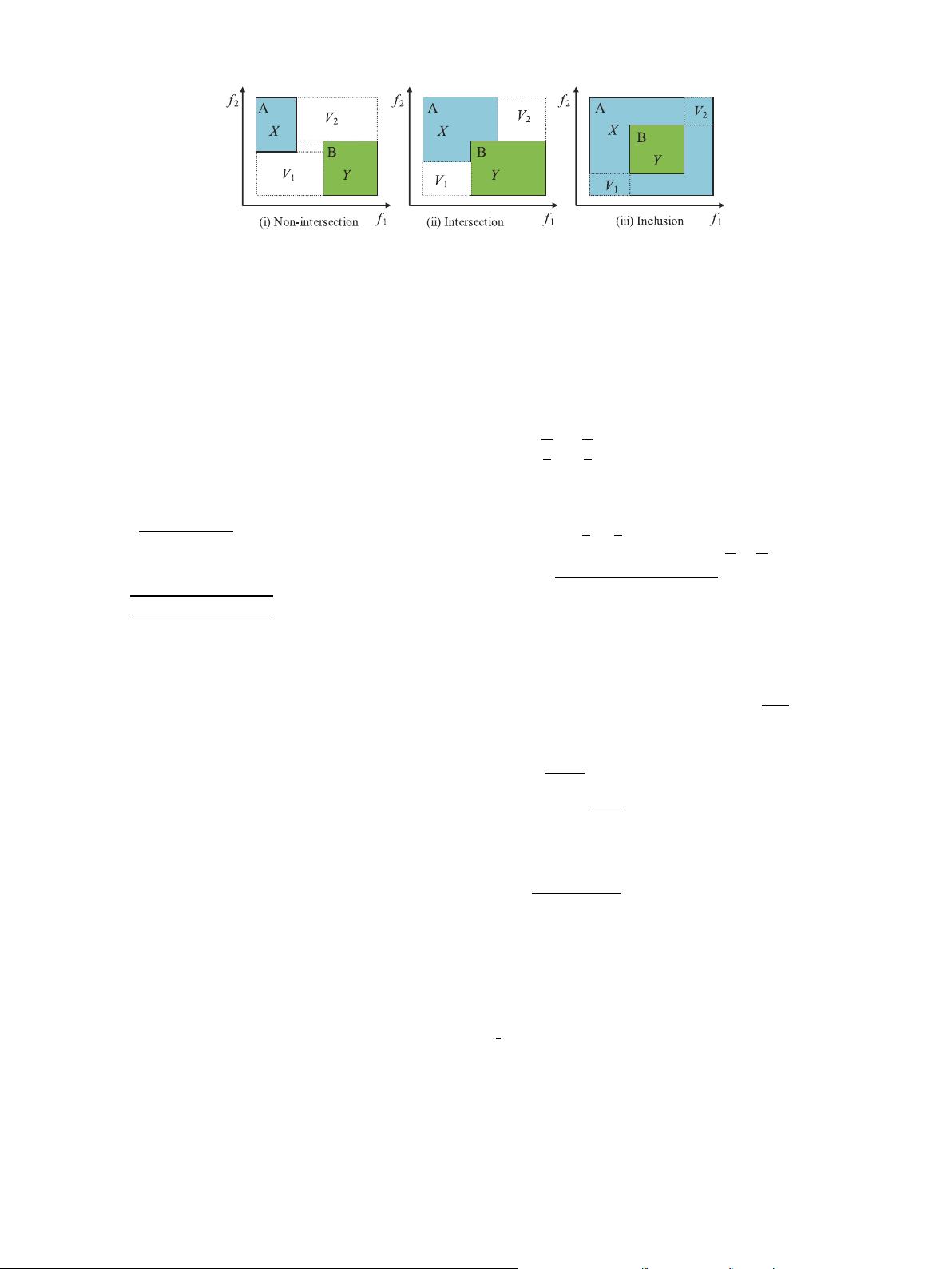
Fig. 1. The relationship between hypercubes of two candidates.
We here introduce the following weak comparison relation between 𝐴
and 𝐵,
𝐴 ≤ 𝐵 ⟺ 𝐴
𝑅
≤ 𝐵
𝐿
, 𝐴 ≥ 𝐵 ⟺ 𝐵 ≤ 𝐴. (2)
Generally speaking, it is not true that 𝐴 − 𝐴 = 0, for example when
A=[−2,2], we can see that A-A=[−4,4]. Thus, we here prescribe that
𝐴 equals 𝐵 if and only if 𝐴
𝐿
= 𝐵
𝐿
and 𝐴
𝑅
= 𝐵
𝑅
. This way, Eq. (2)
indicates that once 𝐴 ≤ 𝐵 and 𝐵 ≤ 𝐴, 𝐴 and 𝐵 will degenerate to 𝑎,
i.e., [𝑎, 𝑎]. It is emphasized that, when 𝐴 ∩ 𝐵 ≠ 𝜙 and 𝐴 ≠ 𝐵, Eq. (2)
cannot be adopted to execute comparison between 𝐴 and 𝐵. In such
case, the version of possibility degree is an alternative way to compare
𝐴 with 𝐵. We here cite the following possibility degree model (Zhou
and Liu, 2008),
𝑃 𝑟{𝐴 ≤ 𝐵} =
𝑑(𝐴, 𝐶)
𝑑(𝐴, 𝐶) + 𝑑(𝐵, 𝐶)
, (3)
where 𝐶 = [𝐶
𝐿
, 𝐶
𝑅
], 𝐶
𝑅
= max Γ and 𝐶
𝐿
= max Γ ⧵ {𝐶
𝑅
} with
Γ = {𝐴
𝐿
, 𝐴
𝑅
, 𝐵
𝐿
, 𝐵
𝑅
}, and meanwhile
𝑑(𝐴, 𝐶) =
(𝐴
𝐿
− 𝐶
𝐿
)
2
+ (𝐴
𝑅
− 𝐶
𝑅
)
2
2
. (4)
Based on Eq. (3), Zhou and Liu (2008) introduced the version of
individual dominance. In other words, 𝐱 dominates 𝐲 (𝐱 ≺ 𝐲) if 𝜎
𝑖
(𝐱, 𝐲) ≥
𝜎
𝑖
(𝐲, 𝐱) for any 𝑖 with 1 ≤ 𝑖 ≤ 𝑚, and there exists 𝑖
0
such that 𝜎
𝑖
0
(𝐱, 𝐲) >
𝜎
𝑖
0
(𝐲, 𝐱), where
𝜎
𝑖
(𝐱, 𝐲) = 𝑃 𝑟{𝑓
𝑖
(𝐱, 𝑈 ) ≤ 𝑓
𝑖
(𝐲, 𝑈 )}. (5)
Naturally, 𝐱
∗
is said to be a Pareto optimal solution of the above MIVP if
there does not exist 𝐲 in 𝐷 such that 𝐲 ≺ 𝐱
∗
. In order to identify whether
one individual is superior to another one in a given population 𝐴 with
size 𝑁, we introduce the following computational model to compute the
rank of individual 𝐱 in 𝐴,
𝑅(𝐱) = 𝑁 − {𝐲 ∈ 𝐴𝐲 ≺ 𝐱}, (6)
where Λrepresents the number of elements in set Λ. Eq. (6) indicates
that 𝐱 is better if 𝑅(𝐱) is larger, and especially it is a non-dominated
individual in 𝐴 if 𝑅(𝐱) = 𝑁 . This way, 𝐴 may be divided into two sub-
populations. One is composed of non-dominated individuals in 𝐴, the
other consists of those dominated ones.
Remark 1. When computing the ranks of all individuals in 𝐴, we
first need to calculate the possibility degrees of sub-objective interval
numbers for any two individuals through Eq. (3), for which the total of
executions is 𝑚𝑁
2
. Second, we also execute 𝑚𝑁
2
comparisons between
individuals through non-dominated sorting. Once all the non-dominated
individuals in 𝐴 need to be discriminated, the computational complexity
is 𝑂(𝑚𝑁
2
).
4. Crowding degree model
As we know, the objective interval vectors of individuals 𝐱 and 𝐲,
i.e., 𝑓 (𝐱, 𝑈) and 𝑓 (𝐲, 𝑈), correspond to two hypercubes in the objective
space. In general, their possible position relations, given by Fig. 1
include non-intersection, intersection and inclusion. In the above figure,
𝑋 and 𝑌 denote the hypercubes of interval objective vectors 𝑓 (𝐱, 𝑈 )
and 𝑓 (𝐲, 𝑈 ) for candidates 𝐱 and 𝐲, respectively; A and B represent the
vertexes of 𝑋 and 𝑌 at the top-left corner, respectively; 𝑉
1
and 𝑉
2
stand
for the hypervolumes of the corresponding dash hypercubes. Let 𝑉
𝑥𝑦
be
the hypervolume of the outer hypercube. In this way, 𝑉
1
, 𝑉
2
and 𝑉
𝑥𝑦
can
be represented by the endpoints of the interval-valued sub-objectives,
𝑉
1
=
𝑚
𝑖=1
𝑓
𝑖
(𝐱) − 𝑓
𝑖
(𝐲),
𝑉
2
=
𝑚
𝑖=1
𝑓
𝑖
(𝐱) − 𝑓
𝑖
(𝐲),
𝑉
𝑥𝑦
=
𝑚
𝑖=1
(𝑐
𝑖
− 𝑑
𝑖
),
(7)
where 𝑐
𝑖
= max{𝑓
𝑖
(𝐱), 𝑓
𝑖
(𝐲)} and 𝑑
𝑖
= min{𝑓
𝑖
(𝐱), 𝑓
𝑖
(𝐲)}. Additionally, the
distance between A and B is defined by
𝑑(𝐱, 𝐲) =
𝑚
𝑖=1
(𝑚(𝑓
𝑖
(𝐱, 𝑈 )) − 𝑚(𝑓
𝑖
(𝐲, 𝑈 )))
2
,
(8)
where 𝑚(𝑓
𝑖
(𝐱, 𝑈 )) denotes the midpoint of interval 𝑓
𝑖
(𝐱, 𝑈 ). Although
Eq. (8) can present the degree of approximation of points A and B,
it cannot completely reflect the relation between the two hypercubes.
Once we move the positions of 𝑋 and 𝑌 , the values of 𝑉
1
, 𝑉
2
, 𝑉
𝑥𝑦
and
𝑑(𝐱, 𝐲) will make change correspondingly, but
𝑉
1
+𝑉
2
2𝑉
𝑥𝑦
only does minor
change. This way, the crowding degree of 𝐱 and 𝐲 in the objective space
can be defined here by
𝐷(𝐱, 𝐲) =
𝑉
1
+ 𝑉
2
2𝑉
𝑥𝑦
𝑑(𝐱, 𝐲). (9)
Again, since 0 ≤
𝑉
1
+𝑉
2
𝑉
𝑥𝑦
< 1, 𝐷(𝐱, 𝐲) changes within 0 and 𝑑(𝐱, 𝐲). Eq.
(9) hints that if 𝑋 and 𝑌 are close, 𝐷(𝐱, 𝐲) is small. Therefore, in order
to reflect the diversity of a given population 𝑃 , the crowding degree of
individual 𝐱 in 𝑃 is designed by
𝐶(𝐱) =
𝐷(𝐲, 𝐱) + 𝐷(𝐱, 𝐳)
2
(10)
where 𝐲 and 𝐳 are two closest individuals of 𝐱 in 𝑃 . Eq. (10) illustrates
that, if the crowding degrees of individuals in 𝑃 are small, these
individuals will have high similarity and thus weak population diversity.
Remark 2. In order to compute the crowding degrees of individuals
in 𝑃 with size 𝑁, the two closest individuals of each individual in
the objective space are first decided, for which we need to execute
(
1
2
𝑁(𝑁 − 1) + 𝑁𝑙𝑜𝑔𝑁 ) times. Thus, once Eq. (10) is enforced in 𝑃 , it
will cause the complexity of 𝑂(𝑁
2
).
5. Algorithm formulation and design
Based on the above designs, immune inspirations and also additive
genetic operators, we in this section formulates MIIGA, for which
the flowchart is given in Fig. 2. One such approach includes three
functional modules, i.e., population division, immune evolution and
237


