使用Halcon 10进行图像分类：GMM、SVM与神经网络算法解析

4星 · 超过85%的资源需积分: 48 85 浏览量更新于2024-08-01 1 收藏 4MB PDF 举报

"Halcon 10 图像分类算法" 在机器视觉领域，Halcon是一种广泛使用的图像处理软件，尤其在图像分类方面具有强大的功能。Halcon 10 提供了多种算法来应对图像分类任务，包括高斯混合模型（GMM）、支持向量机（SVM）以及神经网络。这些算法在不同场景下各有优势，可以根据具体需求选择合适的分类方法。 1. **高斯混合模型（GMM）**： GMM 是一种统计建模技术，它假设数据由多个高斯分布混合而成。在图像分类中，GMM 可用于对像素或特征进行建模，通过学习各个类别的概率分布，将新图像分配到最匹配的类别。GMM 的优点在于它能处理多峰分布，并且在有限的数据集上也能表现良好。 2. **支持向量机（SVM）**： SVM 是一种监督学习模型，其目标是找到一个超平面，最大化不同类别之间的间隔。在图像分类中，SVM 可以通过学习训练样本的特征向量，构建决策边界来区分不同类别。SVM 对于非线性可分问题有很好的处理能力，且在小样本情况下表现优秀。 3. **神经网络**：神经网络是一种模拟人脑神经元结构的计算模型，可以用于图像分类、物体识别等复杂任务。在Halcon 10中，可能包含前馈神经网络和卷积神经网络（CNN）。前馈网络适用于一般的特征学习，而CNN则特别适合图像处理，因为它可以自动学习和提取图像的局部特征。CNN通过多层结构和池化操作，提高了对图像内容的理解能力。在实际应用中，Halcon 提供的这些分类方法不仅限于单独使用，还可以结合使用，以达到更优的分类效果。例如，可以先用SVM初步分类，然后用神经网络进行细粒度分类。用户可以通过调整算法参数、优化网络结构以及选择合适的训练策略，来提升分类的准确性和鲁棒性。 Halcon 的解决方案指南提供了详细的使用教程，指导用户如何配置和训练这些分类算法。用户可以学习如何准备训练数据、设置模型参数、评估模型性能以及如何将模型部署到实际应用中。此外，手册还可能包含实例代码和示例图像，帮助用户快速上手并理解分类过程。对于想要深入了解Halcon 10 图像分类的用户，建议访问官方网址 http://www.halcon.com/ 获取更多详细信息、文档和最新资源，以便更好地利用这些强大的工具解决实际问题。同时，Halcon 还可能涉及到其他专利技术，使用时需遵守相关法律法规。

D-16 Classiﬁcation: Theoretical Background

Figure 3.1: Region features of oranges and lemons are extracted and can be added as samples to the

classiﬁer.

a feature space can have any dimension, depending on the number of features contained in the feature

vector. For visualization purpose, here a 2D feature space is shown. In practice, feature spaces of higher

dimension are very common.

In ﬁgure 3.2 the feature vectors of the fruits shown in ﬁgure 3.1 are visualized in a 2D graph, for which

one axis represents the ’area’ values and the other axis represents the ’circularity’ values. Al-

though the regions vary in size and circularity, we can see that they are similar enough to build clusters.

The goal of a classiﬁer is to separate the clusters and to assign each feature vector to one of the clusters.

Here, the oranges and lemons can be separated, e.g., by a straight line. All objects on the lower left side

of the line are classiﬁed as lemons and all objects on the upper right side of the line are classiﬁed as

oranges.

As we can see, the feature vector of a very small orange and that of a rather circular lemon are close to

the separating line. With a little bit different data, e.g., if the small orange additionally would be less

circular, the feature vectors may be classiﬁed incorrectly. To minimize errors, a lot of different samples

and in many cases also additional features are needed. An additional feature for the citrus fruits may

be, e.g., the gray value. Then, not a line but a plane is needed to separate the clusters. If color images

D-18 Classiﬁcation: Theoretical Background

from each other. In section 6.3 on page 78 it is described how to apply the Euclidean classiﬁer for image

segmentation. With HALCON, the Euclidean metric is used only for image segmentation, not for the

classiﬁcation of general features or OCR. This is because the approach is stable only for feature vectors

of low dimension.

x x

Feature 1:

Feature 2:

Figure 3.3: Euclidean classiﬁer.

Whereas the Euclidean classiﬁer uses n-dimensional spheres, the hyperbox approach uses axis-parallel

cubes, so-called hyperboxes. This can be imagined as a threshold approach in multidimensional space.

That is, for each class speciﬁc value ranges for each axis of the feature space are determined. If a feature

vector lies within all the ranges of a speciﬁc class, it will be assigned to this class. The hyperboxes can

overlap. For objects that are ambiguous, the hyperbox approach can be combined with another classiﬁ-

cation approach, e.g., an Euclidean classiﬁcation or a maximum likelihood classiﬁcation. Within HAL-

CON, the Euclidean distance is used and additionally weighted with the variance of the feature vector.

In section 6.3 on page 78 it is described how to apply the hyperbox classiﬁer for image segmentation.

HALCON provides also operators for hyperbox classiﬁcation of general features as well as for OCR,

but these show almost no advantages but a lot of disadvantages compared to the MLP, SVM, and GMM

approaches, and thus are not described further in this solution guide.

3.3 Gaussian Mixture Models (GMM)

The classiﬁcation approaches described in section 3.2 on page 17 followed rather simple rules. The

theory for the classiﬁcation with Gaussian mixture models (GMM) is a bit more complex, so we have to

deal with the theory of classiﬁcation in more detail.

One of the basic theories when dealing with classiﬁcation comprises the Bayes decision rule. Generally,

the Bayes decision rule tells us to minimize the probability of erroneously classifying a feature vector

by maximizing the probability for the feature vector x to belong to a class. This so-called ’a posteriori

probability’ should be maximized over all classes. Then, the Bayes decision rule partitions the feature

space into mutually disjoint regions. The regions are separated by hypersurfaces, e.g., by points for 1D

D-20 Classiﬁcation: Theoretical Background

The second problem of the Bayes classiﬁer is how to obtain the a priori probability P (x|w_i). In prin-

ciple, a histogram over all feature vectors of the training set can be used. The apparent solution is to

subdivide each dimension of the feature space into a number of bins. But as the number of bins grows

exponentially with the dimension of the feature space, you face the so-called ’curse of dimensionality’.

That is, to get a good approximation for P (x|w_i), you need more memory than can be handled properly.

With another solution, instead of keeping the size of a bin constant and varying the number of samples in

the bin, the number of samples k for a class w_i is kept constant while varying the volume of the region

in space around the feature vector x that contains the k samples (v(x, w_i)). The volume depends on the

k nearest neighbors of the class w_i, so the solution is called k nearest-neighbor density estimation. It

has the disadvantage that all training samples have to be stored with the classiﬁer and the search for the k

nearest neighbors is rather time-consuming. Because of that, it is seldom used in practice. A solution that

can be used in practice assumes that P (x|w_i) follows a certain distribution, e.g., a normal distribution.

Then, you only have to estimate the two parameters of the normal distribution, i.e., the mean vector µ_i

and the covariance matrix Σ_i. This can be achieved, e.g., by a maximum likelihood estimator.

In some cases, a single normal distribution is not sufﬁcient, as there are large variations inside a class.

The character ’a’, e.g., can be represented by ’a’ or ’a’, which have signiﬁcantly different shapes. Nev-

ertheless, both belong to the same character, i.e., to the same class. Inside a class with large variations, a

mixture of l_i different densities exists. If these are again assumed to be normal distributed, we have a

Gaussian mixture model. Classifying with a Gaussian mixture model means to estimate to which speciﬁc

mixture density a sample belongs. This is done by the so-called expectation minimization algorithm.

Coarsely spoken, the GMM classiﬁer uses probability density functions of the individual classes and

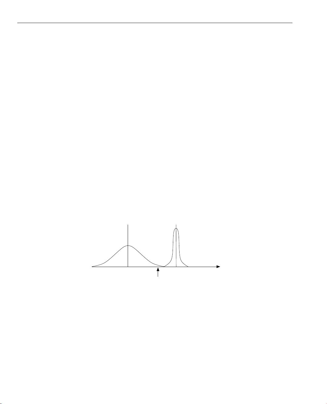
expresses them as linear combinations of Gaussian distributions (see ﬁgure 3.5). Comparing the approach

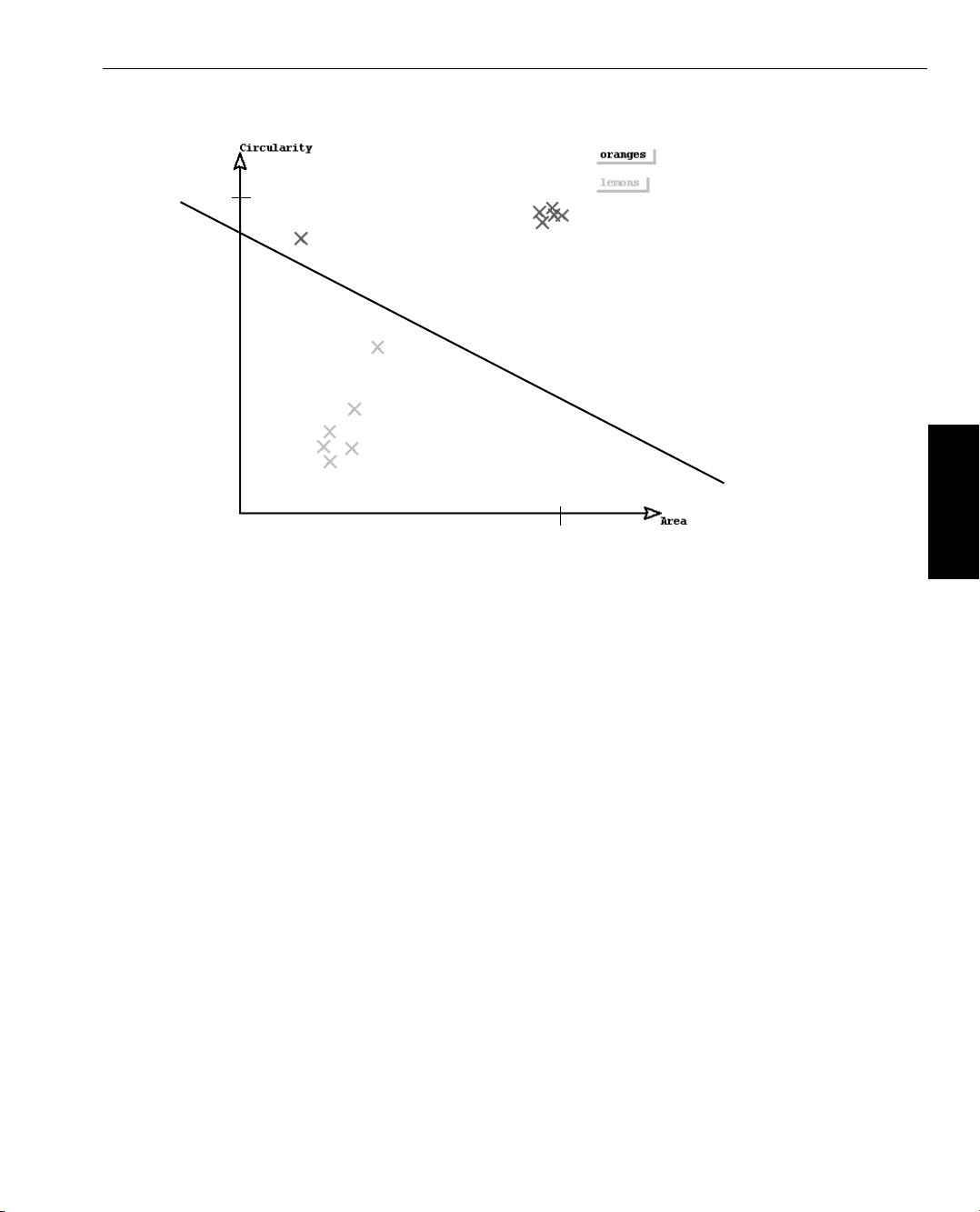
to the simple classiﬁcation approaches described in section 3.2 on page 17, you can imagine the GMM

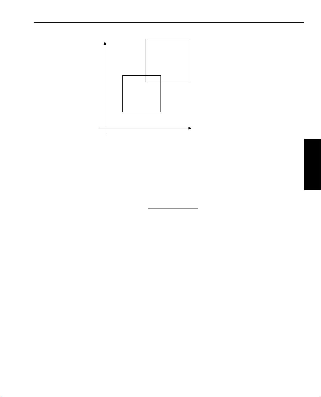
to construct n-dimensional error (covariance) ellipsoids around the cluster centers (see

ﬁgure 3.6).

Feature Vector X

Feature Vectors

Class 1 Class 2

Figure 3.5: The variance of class 1 is signiﬁcantly larger than that of class 2. In such a case, the distance

to the Gauss error distribution curve is a better criteria for the class membership than the

distance to the cluster center.

GMM are reliable only for low dimensional feature vectors (approximately up to 15 features), so HAL-

CON provides GMM only for the classiﬁcation of general features and image segmentation, but not for

OCR. Typical Applications are image segmentation and novelty detection. Novelty detection is speciﬁc

for GMM and means that feature vectors that do not belong to one of the trained classes can be rejected.

Note that novelty detection can also be applied with SVM, but then a speciﬁc parameter has to be set and

only two-class problems can be handled, i.e., a single class can be trained and the feature vectors that do

not belong to that single class are rejected.

There are two general approaches for the construction of a classiﬁer. First, you can estimate the a pos-

剩余115页未读，继续阅读

starluckwang

粉丝: 0
资源: 2

使用Halcon 10进行图像分类：GMM、SVM与神经网络算法解析

Halcon 深度学习分类模型介绍

Halcon视觉检测——使用分类器分类

Halcon SVM分类使用图片

halcon缺陷检测的算法流程.txt

Halcon图像匹配算法总结与应用场景解析

halcon中，抽色算法

HALCON算法.pdf

halcon18.11图像处理库

halcon深度学习分类系统开发流程详解

halcon深度学习算法

最新资源