基于稀疏表示的鲁棒人脸识别方法

5星 · 超过95%的资源需积分: 43 147 浏览量更新于2024-07-27 3 收藏 3.04MB PDF 举报

"Robust Face Recognition via Sparse Representation" 是一篇关注人脸识别技术的学术论文，由John Wright、Allen Y. Yang、Arvind Ganesh、S. Shankar Sastry和Yi Ma等多位IEEE会员共同撰写。论文的核心观点是将人脸识别问题视为在多个线性回归模型间进行分类，并强调了稀疏信号表示理论在解决这个问题中的关键作用。通过1-范数最小化方法计算得到的稀疏表示，作者提出了一种通用的基于图像的对象识别算法。在这个新框架下，论文探讨了人脸识别中的两个关键挑战：特征提取和对遮挡的鲁棒性。首先，作者指出，以往对于特征选择的依赖度降低，因为当正确地利用稀疏性时，特征选择的重要性变得不那么显著。然而，特征的数量是否足够以及稀疏表示的准确性成为了新的关注点。这意味着在设计算法时，不仅要关注特征选择的质量，还要确保有足够的特征来捕捉人脸的复杂性，并且算法应能处理不同表情、光照条件下的变化，以及面部遮挡的情况。此外，论文可能还探讨了如何通过稀疏编码技术（如非负矩阵分解或者稀疏编码器）来提取人脸的特征向量，这些特征向量能够有效地压缩并保留人脸的识别关键信息，即使在存在噪声或遮挡的情况下也能保持较高的识别精度。这种鲁棒性是通过减少冗余信息和增强对异常模式的抵抗实现的。为了实现算法的实用性，文中可能会提供具体的实现步骤和实验结果，包括训练数据集的选择、特征提取和降维技术、以及与传统方法（如PCA、LDA等）的性能比较。可能还会讨论如何通过迭代优化算法（如ISTA或ADMM）求解1-范数最小化问题，以找到最合适的稀疏表示。这篇论文将稀疏表示理论应用于人脸识别领域，提出了一个创新的分类框架，强调了稀疏性在特征提取和应对遮挡等复杂情况下的优势。其研究不仅推动了人脸识别技术的发展，也为其他领域的信号处理提供了新的思考角度。如果提供了代码，读者可以借此深入理解并实现这一鲁棒的稀疏表示人脸识别算法。

As the entries of the vector xx

encode the identity of the

test sample yy, it is tempting to attempt to obtain it by

solving the linear system of equations yy ¼ Axx. Notice,

though, that using the entire training set to solve for xx

represents a significant departure from one sample or one

class at a time methods such as NN and NS. We will later

argue that one can obtain a more discriminative classifier

from such a global representation. We will demonstrate its

superiority over these local methods (NN or NS) both for

identifying objects represented in the training set and for

rejecting outlying samples that do not arise from any of the

classes present in the training set. These advantages can

come without an increase in the order of growth of the

computation: As we will see, the complexity remains linear

in the size of training set.

Obviously, if m>n, the system of equations yy ¼ Axx is

overdetermined, and the correct xx

can usually be found as

its unique solution. We will see in Section 3, however, that

in robust face recognition, the system yy ¼ Axx is typically

underdetermined, and so, its solu tion is not unique.

Conventionally, this difficulty is resolved by choosing the

minimum ‘

-norm solution:

ð‘

Þ :

¼ arg min kxxk

subject to Axx ¼ yy: ð4Þ

While this optimization problem can be easily solved (via

the pseudoinverse of A), the solution

is not especially

informative for recognizing the test sample yy. As shown in

Example 1, ^xx

is generally dense, with large nonzero entries

corresponding to training samples from many different

classes. To resolve this difficulty, we instead exploit the

following simple observation: A valid test sample yy can be

sufficiently represented using only the training samples

from the same class. This representation is naturally sparse if

the number of object classes k is reasonably large. For

instance, if k ¼ 20, only 5 percent of the entries of the

desired xx

should be nonzero. The more sparse the

recovered xx

is, the easier will it be to accurately determine

the identity of the test sample yy.

This motivates us to seek the sparsest solution to yy ¼ Axx,

solving the following optimization problem:

ð‘

Þ :

¼ arg min kxxk

subject to Axx ¼ yy; ð5Þ

where kk

denotes the ‘

-norm, which counts the number

of nonzero entries in a vector. In fact, if the columns of A are

in general position, then whenever yy ¼ Axx for some xx with

less than m=2 nonzeros, xx is the unique sparsest solution:

¼ xx [33]. However, the problem of finding the sparsest

solution of an underdetermined system of linear equations is

NP-hard and difficult even to approximate [13]: that is, in the

general case, no known procedure for finding the sparsest

solution is significantly more efficient than exhausting all

subsets of the entries for xx.

2.2 Sparse Solution via ‘

-Minimization

Recent development in the emerging theory of sparse

representation and compressed sensing [9], [10], [11] reveals

that if the solution xx

sought is sparse enough, the solution of

the ‘

-minimization problem (5) is equal to the solution to

the following ‘

-minimization problem:

ð‘

Þ :

¼ arg min kxxk

subject to Axx ¼ yy: ð6Þ

This problem can be solved in polynomial time by standard

linear programming methods [34]. Even more efficient

methods are available when the solution is known to be

very sparse. For example, homotopy algorithms recover

solutions with t nonzeros in Oðt

þ nÞ time, linear in the size

of the training set [35].

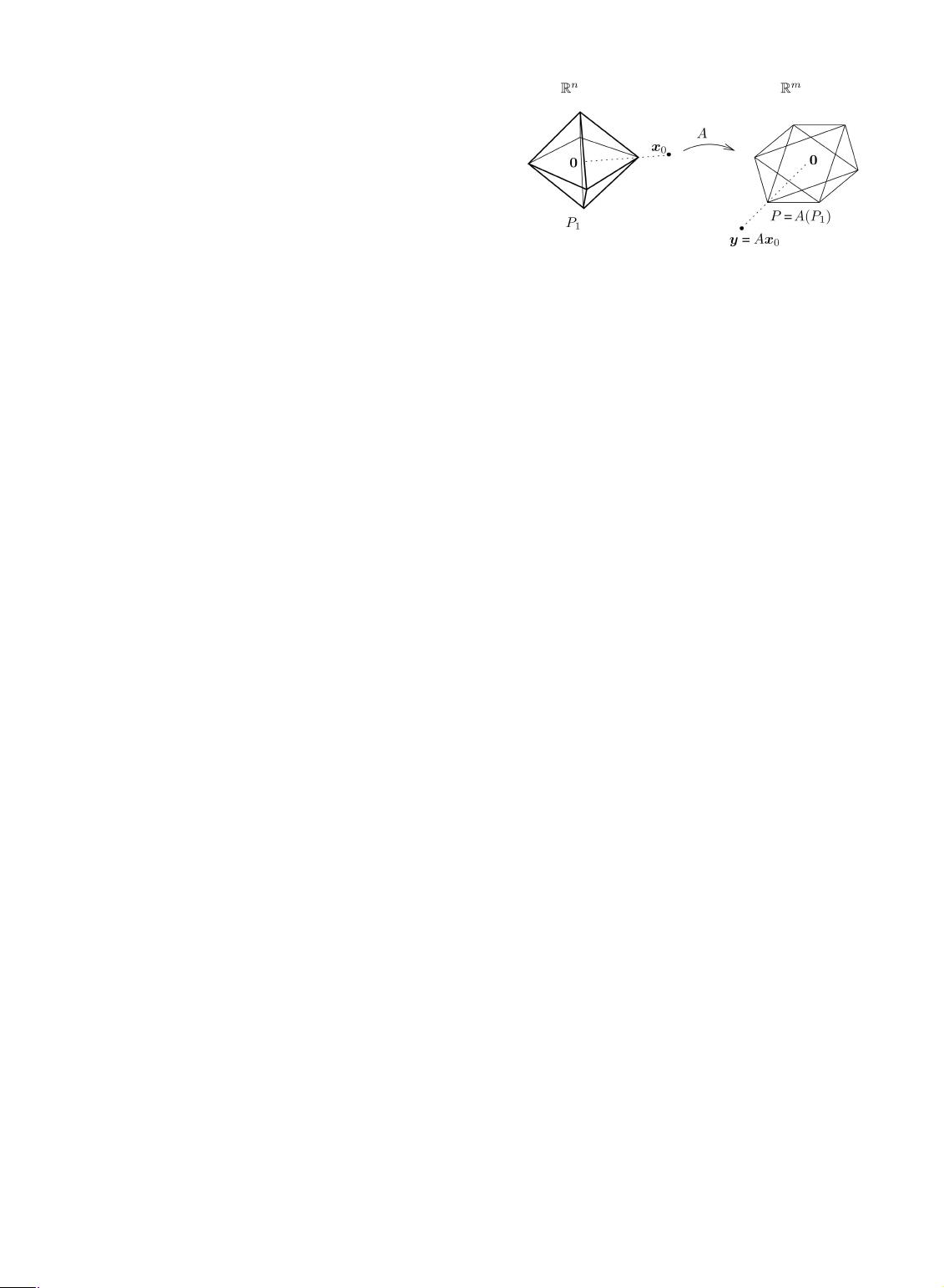
2.2.1 Geometric Interpretation

Fig. 2 gives a geometric interpretation (essentially due to

[36]) of why minimizing the ‘

-norm correctly recovers

sufficiently sparse solutions. Let P



denote the ‘

-ball (or

crosspolytope) of radius :



fxx : kxxk

 gIR

: ð7Þ

In Fig. 2, the unit ‘

-ball P

is mapped to the polytope

P¼

AðP

ÞIR

, consisting of all yy that satisfy yy ¼ Axx for

some xx whose ‘

-norm is  1.

The geometric relationship between P



and the polytope

AðP



Þ is invariant to scaling. That is, if we scale P



, its

image under multiplication by A is also scaled by the same

amount. Geometrically, finding the minimum ‘

-norm

solution

to (6) is equivalent to expanding the ‘

-ball P



until the polytope AðP



Þ first touches yy. The value of  at

which this occurs is exactly k

Now, suppose that yy ¼ Axx

for some sparse xx

. We wish

to know when solving (6) correctly recovers xx

.This

question is easily resolved from the geometry of that in

Fig. 2: Since

is found by expanding both P



and AðP



until a point of AðP



Þ touches yy, the ‘

-minimizer

must

generate a point A

on the boundary of P .

Thus,

¼ xx

if and only if the point Aðxx

=kxx

Þ lies on

the boundary of the polytope P. For the example shown in

Fig. 2, it is easy to see that the ‘

-minimization recovers all

with only one nonzero entry. This equivalence holds

because all of the vertices of P

map to points on the

boundary of P.

In general, if A maps all t-dimensional facets of P

facets of P , the polytope P is referred to as (centrally)

t-neighborly [36]. From the above, we see that the

‘

-minimization (6) correctly recovers all xx

with  t þ 1

nonzeros if and only if P is t-neighborly, in which case, it is

WRIGHT ET AL.: ROBUST FACE RECOGNITION VIA SPARSE REPRESENTATION 213

Fig. 2. Geometry of sparse representation via ‘

-minimization. The

‘

-minimization determines which facet (of the lowest dimension) of the

polytope AðP



Þ, the point yy=kyyk

lies in. The test sample vector yy is

represented as a linear combination of just the vertices of that facet, with

coefficients xx

6. Furthermore, even in the overdetermined case, such a linear equation

maynotbeperfectlysatisfiedinthepresenceofdatanoise(see

Section 2.2.2).

7. This intuition holds only when the size of the database is fixed. For

example, if we are allowed to append additional irrelevant columns to A,

we can make the solution xx

have a smaller fraction of nonzeros, but this

does not make xx

more informative for recognition.

剩余17页未读，继续阅读

shuanger1233

粉丝: 0
资源: 2

基于稀疏表示的鲁棒人脸识别方法

Robust Face Recognition via Sparse Representation

robust face recognition algorithm

ArcFace: Additive Angular Margin Loss for Deep Face Recognition

PAMI-Robust FaceRecognition via Sparse Representation

Low-rank constrained collaborative representation for robust face recognition

Iterative Re-constrained Group Sparse Face Recognition

Sparse Alignment for Robust Tensor Learning

stacked convolutional sparse denoising autoencoder

【含数据库+附源码+说明文档】基于Java swing和mysql实现的银行管理系统（彩色版本）

计算机原理之什么是重定位

最新资源