深度学习解析：从监督到无监督

需积分: 5 10 浏览量更新于2024-06-27 2 收藏 71.31MB PDF 举报

"理解深度学习" 本书《Understanding DeepLearning》由Simon J.D. Prince撰写，旨在深入探讨深度学习这一主题。作者在2022年12月15日发布了此预览版，最终版本预计将于2024年由麻省理工学院出版社（MIT Press）正式发布。所有关于版权的询问应直接向MIT Press的版权和许可部门提出。本书遵循Creative Commons CC-BY-NC-ND许可协议，并欢迎读者提供反馈和建议。本书内容涵盖了深度学习的基础与核心概念，以帮助读者深入理解这一领域。作者首先介绍了监督学习，这是机器学习的一个主要分支。监督学习包括回归和分类问题，其中，回归问题涉及预测连续值，而分类问题则涉及预测离散类别。输入数据在模型中起着关键作用，它可以是各种形式，如图像、文本或数值数据。接着，书中详细讨论了机器学习模型，特别是深度神经网络（DNNs）。深度学习的“深度”来源于其多层结构，这些层次允许模型学习复杂的特征表示。DNNs在图像识别、自然语言处理和许多其他领域都表现出卓越的性能。在监督学习之后，Prince转向了无监督学习。无监督学习不依赖于标记数据，它通常用于发现数据中的模式和结构。书中特别提到了生成模型，这类模型可以学习数据的概率分布，并用来生成新的、类似的数据样本。另一个无监督学习的子领域是聚类，尽管在书中未详细展开，但它同样重要，能帮助我们发现数据的内在结构和群体。此外，书中还提及了结构化输出，这是一个关键概念，特别是在处理序列数据或需要生成复杂结构（如语法树或图像布局）的任务时。结构化输出的学习通常涉及更复杂的损失函数和解码策略。《Understanding DeepLearning》是一本面向深度学习初学者和专业人士的详细教程，它不仅涵盖基础概念，还深入到监督和无监督学习的实践应用，以及深度神经网络的关键特性。通过阅读这本书，读者将能够更好地理解深度学习的原理，以及如何在实际项目中应用这些原理。

12 1 Introduction

Figure 1.1 Machine learning is an area

of articial intelligence that ts math-

ematical models to observed data. It

can coarsely be divided into supervised

learning, unsupervised learning, and re-

inforcement learning. Deep neural net-

works contribute to each of these areas.

1.1.1 Regression and classication problems

Figure 1.2 depicts several regression and classication problems. In each case, there is a

meaningful real-world input (a sentence, a sound le, an image, etc.) and this is encoded

as a vector of numbers. This vector forms the input to the model. The model maps the

input to an output vector and this is then “translated” back to a meaningful real-world

prediction. For now, we’ll focus on the inputs and outputs and just treat the model as

a black box that ingests a vector of numbers and returns another vector of numbers.

The model in gure 1.2a predicts the price of a house based on input characteristics

like the square footage and number of bedrooms. This is a univariate regression problem;

it is a regression problem because the model returns a continuous number (rather than

a category assignment). It is univariate because it only returns one such number. In

contrast, the model in 1.2b takes the chemical structure of a molecule as an input and

predicts both the melting and boiling points. This is a multivariate regression problem

since it predicts more than one real number.

The model in gure 1.2c receives a text string containing a restaurant review as input

and predicts whether the review is positive or negative. This is a binary classication

problem because the model attempts to assign the input to one of two categories. The

output vector contains the probabilities that the input belongs to each category.

Figures 1.2d and 1.2e depict multi-class classication problems. Here, the model

assigns the input to one of K > 2 categories. In the rst case, the input is an audio le

and the model predicts which genre of music it belongs to. In the second case, the input

is an image and the model predicts which object it contains. In each case, the model

returns a xed-length vector that contains the probabilities of each category.

1.1.2 Inputs

The input data in gure 1.2 varies widely. In the house pricing example, the input is a

xed-length vector containing values that characterize the property. This is an example

of tabular data because it has no internal structure; if we change the order of the inputs

and build a new model, then we expect the model prediction to remain the same.

Conversely, the input in the restaurant review example is a body of text. This may

This work is subject to a Creative Commons CC-BY-NC-ND license. (C) MIT Press.

14 1 Introduction

Figure 1.3 Machine learning model. The model represents a family of relationships

that relate the input (age of child) to the output (height of child). The particular

relationship is chosen using training data, which consists of input/output pairs

(orange points). When we train the model, we search through the possible re-

lationships for one that describes the data well. Here, the trained model is the

cyan curve and can be used to compute the height for any age.

be of variable length depending on the number of words in the review, and here input

order is important; my wife ate the chicken is not the same as the chicken ate my wife.

The text must be encoded into numerical form before it can be passed to the model.

Here, we use a xed vocabulary of size 10,000 and simply concatenate the word indices.

For the music classication example, the input vector might be of xed size (perhaps

a 10-second clip) but is very high-dimensional. Digital audio is usually sampled at 44.1

kHz and represented by 16-bit vectors, so a ten-second clip consists of 441, 000 integers.

Clearly, machine learning models will have to be able to process sizeable inputs. The

input in the image classication example (which consists of the concatenated RGB values

at every pixel) is also enormous. Moreover, its structure is naturally two-dimensional;

two pixels that are above and below one another are closely related, even if they are not

adjacent in the input vector.

Finally, the input for the model that predicts the molecule melting and boiling points

is more complex still. The structure of every molecule is dierent; there are varying

numbers of atoms that can be connected in dierent ways. In this case, we must pass

both the structure of the molecule and the constituent components (atoms) to the model.

1.1.3 Machine learning models

Until this point, we have treated the machine learning model as a black box, that takes

an input vector and returns an output vector. But what exactly is in this black box?

This work is subject to a Creative Commons CC-BY-NC-ND license. (C) MIT Press.

1.1 Supervised learning 15

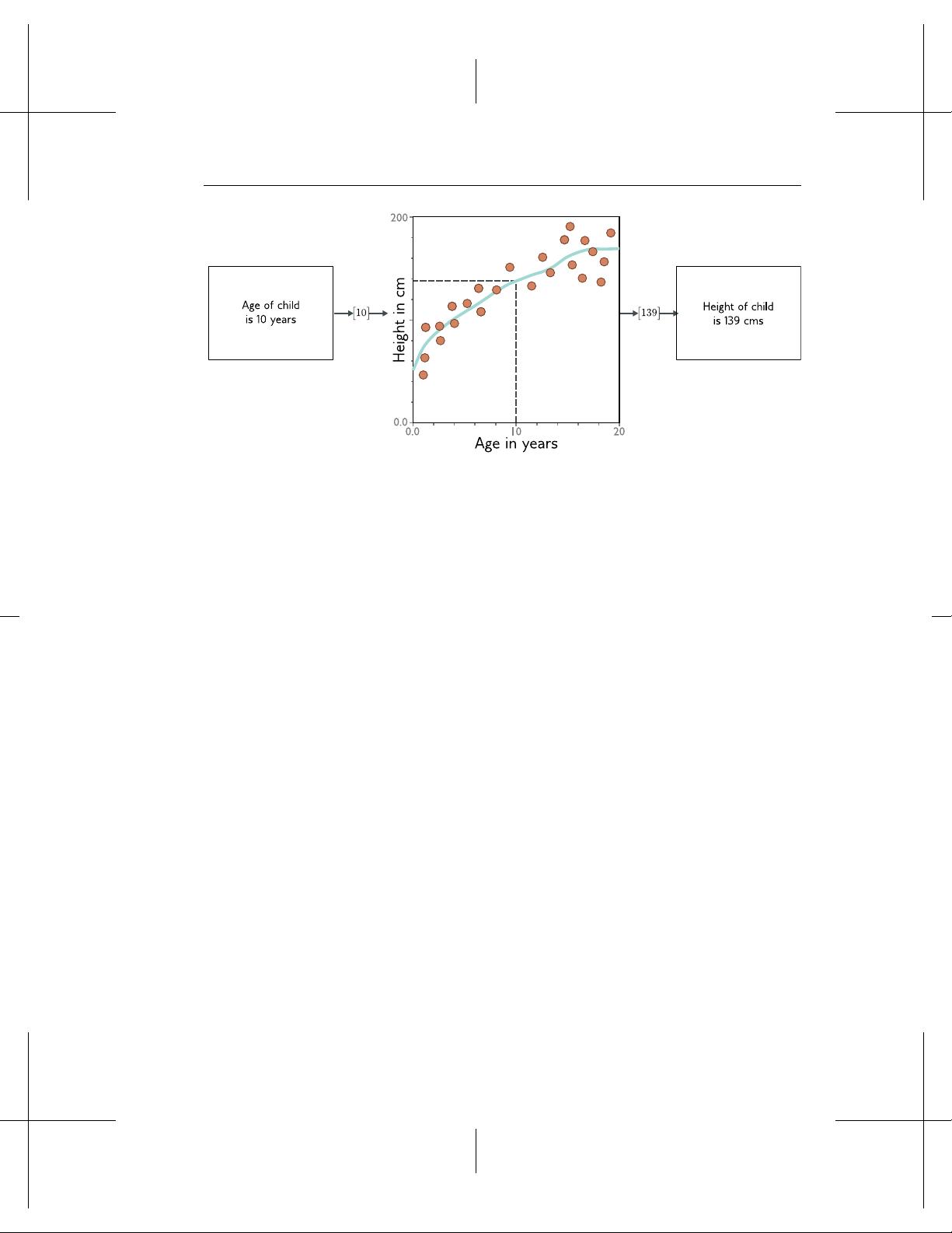
Consider a model to predict the height of a child from their age (gure 1.3). The machine

learning model is a mathematical equation that describes how the average height varies

as a function of age (cyan curve in gure 1.3). When we run the age through this

equation, it returns the height. For example, if the age is 10 years, then we predict that

the height will be 139 cm.

More precisely, the model represents a family of equations mapping the input to

the output (i.e., a family of dierent cyan curves). The particular equation (curve) is

chosen using training data (examples of input/output pairs). In gure 1.3 these pairs

are represented by the orange points and we can see that the model (cyan line) describes

this data reasonably. When we talk about training or tting a model, we mean that we

search through the family of possible equations (possible cyan curves) relating input to

output to nd the one that describes the training data most accurately.

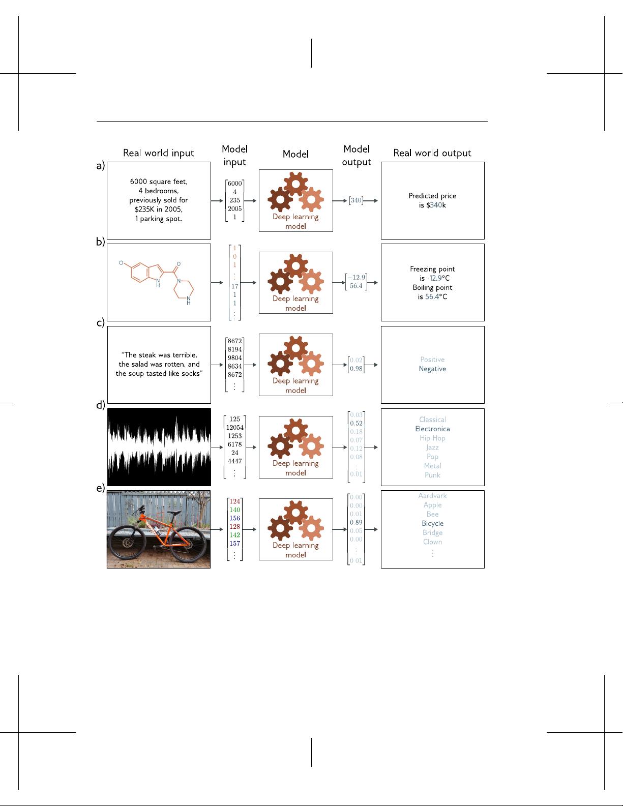
It follows that the models in gure 1.2 require labeled input/output pairs for training.

For example, the music classication model would require a large number of audio clips

where the genre of each had been identied by a human expert. These input/output

pairs take the role of a teacher or supervisor for the training process and this gives rise

to the term supervised learning.

1.1.4 Deep neural networks

This book concerns deep neural networks, which are a particularly useful type of machine

learning model. They are equations that can represent an extremely broad family of

relationships between input and output, and where it is particularly easy to search

through this family to nd the relationship that describes the training data.

Deep neural networks can process inputs that are very large, of variable length,

and contain various kinds of internal structure. They can output single numbers (for

univariate regression), multiple numbers (for multivariate regression), or probabilities

over two or more classes (for binary and multi-class classication, respectively). As we

shall see in the next section, their outputs may also be very large, of variable length,

and contain internal structure. It is probably hard to imagine equations with these

properties; the reader should endeavor to suspend disbelief for now.

1.1.5 Structured outputs

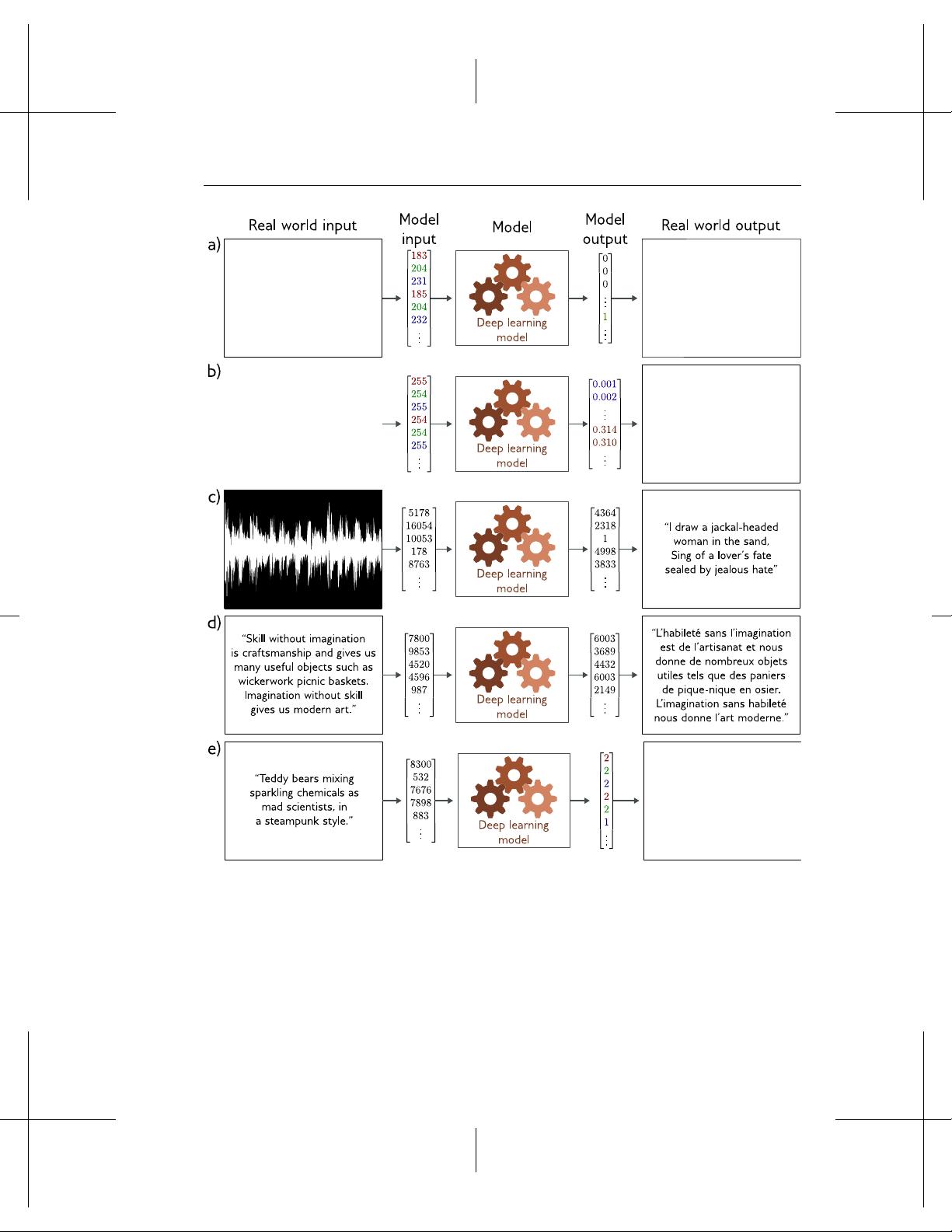
Figure 1.4a depicts a multivariate binary classication model for semantic segmentation.

Here, every pixel of an input image is assigned a binary label that indicates whether it

belongs to a cow or the background. Figure 1.4b shows a multivariate regression model

where the input is an image of a street scene and the output is the depth at each pixel.

In both cases, the output is high-dimensional and structured. However, this structure is

closely tied to the input and this can be exploited; if a pixel is labeled as “cow”, then a

neighbor with a similar RGB value probably has the same label.

Figures 1.4c-e depict three models where the output has a complex structure that is

not so closely tied to the input. Figure 1.4c shows a model where the input is an audio

Draft: please send errata to udlbookmail@gmail.com.

剩余409页未读，继续阅读

asd8705

粉丝: 120
资源: 3

深度学习解析：从监督到无监督

Understanding Deep Learning

Understanding Deep Learning Techniques for Image Segmentation.pdf

deeplearning学习

DeepLearning

Deep Learn

understanding deep learning

Understanding Deep Learning Requires Rethinking Generalization - 2016 (1611.03530v1)-计算机科学

Geometric Understanding of Deep Learning

Deep learning for visual understanding : A review

Python Deep Learning: Exploring deep learning techniques, neural network

最新资源