两帧深度排序：运动分割与通用运动视频的创新算法

需积分: 9 18 浏览量更新于2024-11-06 收藏 546KB PDF 举报

本文主要探讨了一种新颖的视频处理技术——基于遮挡检测器的运动分割与深度排序方法。该研究发表在《Pattern Analysis and Machine Intelligence》杂志上，其标题为"Motion Segmentation and Depth Ordering Using an Occlusion Detector"。论文的作者是Doron Feldman和Daphna Weinshall，他们都是IEEE计算机学会的成员。论文的核心内容分为两部分。首先，作者提出了一种利用空间-时间域的差分特性及尺度空间集成来进行运动分割的方法。这种方法旨在识别视频序列中不同运动区域的边界，通过分析帧与帧之间的运动差异来确定各个区域的动态特性。接着，针对运动边界，文章设计了两种算法来处理两种和三种帧的深度排序问题。值得注意的是，该方法的一大创新之处在于仅依赖于两帧就能进行深度排序，这极大地简化了深度信息的计算过程。这种技术在处理一般运动场景下的六段实际视频序列时展现出良好的效果，表明其在实际应用中的实用性。为了验证算法的鲁棒性，研究者还利用合成数据展示了对高噪声和光照变化的抵抗能力。此外，实验还包括了运动边界处无强度边缘存在的情况，以及无法用参数化运动模型描述的数据，这些测试都证明了算法的有效性。论文的最后部分，作者通过心理物理学实验揭示了一个有趣的现象：人类，就像他们的算法一样，也能仅从两帧中推断出深度顺序，即使单帧中没有明显分层边界的视觉线索。这进一步强化了运动分割和深度排序在人类视觉认知中的作用，并暗示了其潜在的人机交互价值。这项研究不仅提供了一种先进的计算机视觉技术，还在理论和实践上对运动分割和深度排序问题进行了深入探讨，对于视频分析、运动理解以及深度感知等领域具有重要的理论和应用意义。

(a) (b)

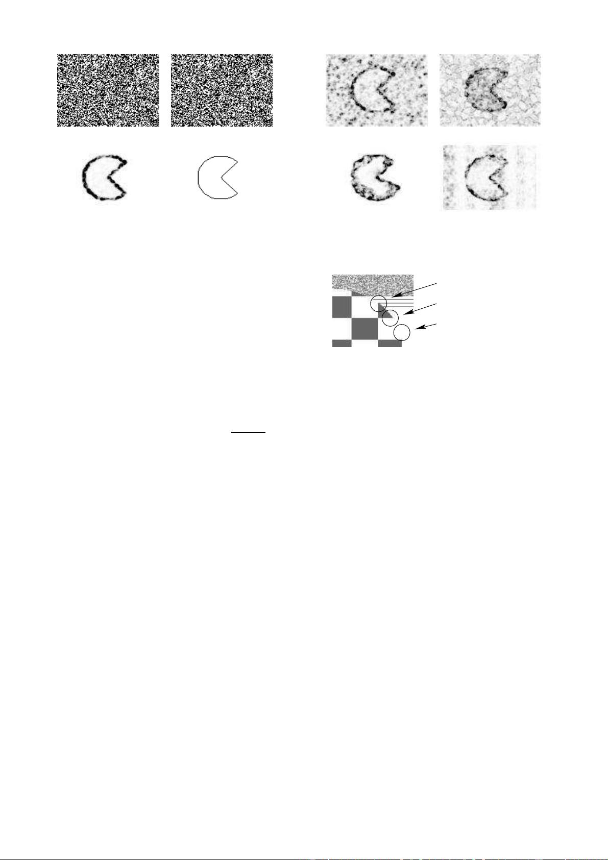
Fig. 1. Random dots example. A shape is moving sideways, where both

the shape and the background are covered by a random pattern of black and

white dots. It is impossible to identify the moving object from each of the two

frames (a) and (b) (a stereo pair) alone. The occlusion detector (c) (higher

values of λ are darker) shows the outline of the object very clearly. Compare

to the ground truth (d).

Velocity-adapted detector: Although rotational invariance is

desirable in the spatial domain, non-spatial rotations in the spatio-

temporal domain have no physical meaning. It is preferable to

have invariance to spatially-ﬁxed shear transformations, which

correspond to 2D relative translational motion between the camera

and the scene. As suggested in [15] by the reference to Galilean

diagonalization, one can use the velocity-adapted matrix

G given

G =





0 0 λ





where λ

det(G)

det(G

∗

)

(3)

denote the entries of G, and G

∗

denotes the 2 ×2 upper-left

submatrix of G containing only spatial information).

Deﬁnition 2: The operator λ

is the velocity-adapted occlu-

sion detector.

To justify this deﬁnition, observe that

G is also invariant to

translation and spatial rotation. The entry λ

is an eigenvalue of

G, and it has been suggested that it encodes the temporal varia-

tion, being the “residue” unexplained by pure-spatial information.

In practice, λ

gives results similar to λ, though it has certain

advantages, as discussed in Section 4. Throughout this paper we

use λ to denote either operator, unless stated otherwise.

Detector effectiveness: High values of λ indicate signiﬁcant

deviation from (2), which is often due to the existence of a motion

boundary. Other sources of large deviations include changes in

illumination (violation of the brightness constancy assumption),

or when the motion varies spatially (motion is not constant in ω).

However, often these events lead to smaller λ values as compared

with motion boundaries (see Fig. 2), in which case the boundary

response can be distinguished from a false response (e.g., by

thresholding).

Low values of λ do not necessarily indicate that the motion

in ω is uniform. The rank of G is affected by spatial structure

as well as temporal structure, so λ may be low even at motion

boundaries, when certain spatial degeneracies exist. Speciﬁcally,

this occurs when there is local ambiguity, i.e., when the existence

of a motion boundary cannot be determined locally. This includes

(a) (b)

Fig. 2. False λ response. The same example as in Fig. 1: (a) with 20%

white noise; (b) with illumination change of 5%; (c) with the object rotating

by 20

◦

; (d) with both object and background patterns deformed smoothly.

linear background

uniform background

same−color background

Fig. 3. Areas where the λ detector is likely to give low values despite the

existence of a local motion boundary.

areas where the occluding object and its background are of the

same color, areas where the background is uniform in color, and

areas where the background texture is uniform in the direction of

the motion (Fig. 3). In the ﬁrst case the rank of G is 0, and in

the other cases the rank of G may be 1 or 2, depending on the

appearance of the occluding object (recall that the λ detector is

high when the rank of G is 3). In these cases, the background

may be interpreted as part of the moving object, since no features

in the background appear to vanish due to occlusion.

2.2. Extraction of Motion Boundaries and Scale Space Structure

The response of λ to occlusion occurs only where some

background features become occluded. Clearly boundary location

cannot always be inferred on the basis of local information alone.

However, while there may be no cues to indicate the location of

the boundary at a ﬁne scale, there may be enough information at a

coarser scale (i.e., in a larger neighborhood) and λ may respond.

Thus we incorporate a multi-scale element in our algorithm, in

order to detect motion boundaries that are not detectable at ﬁne

scales.

Deﬁning scale: In order to deﬁne the notion of scale in

our algorithm, note that the evaluation of λ involves Gaussian

convolutions in two different stages – during the estimation of

the partial derivatives, and when taking the average over the

neighborhood ω. In both cases, larger Gaussians lead to coarser

structures, and we refer to the size of the Gaussian as the scale.

In this work we only consider the spatial scale. As we show in

Appendix I, these two scales are related, and we deﬁne a uniﬁed

scale dimension, and a scaling-invariant operator λ

(s)

at any scale

s > 0, using scale-normalization.

剩余13页未读，继续阅读

writeshadow

粉丝: 1
资源: 11

两帧深度排序：运动分割与通用运动视频的创新算法

Submodular Trajectories for Better Motion segmentation in videos.pdf

Customer Segmentation and Clustering using SAS EM

Global motion segmentation method and application to progressive scanning conversion

Motion Estimation Using Region-Level Segmentation and EKF for AD

An integrated scheme of arbitrarily shaped segmentation and motion estimation

Foreground object extraction through motion segmentation

Segmentation using Thresholding:Segmentation using Thresholding by using inbuilt Matlab functions-matlab开发

matlab精度检验代码-Semantic-Motion-Segmentation-using-Optical-flow-and-Convol

Masseter segmentation using an improved watershed algorithm

计算机视觉大牛Brox的几篇前沿论文optical flow estimation, motion segmentation

最新资源