Mamba：线性时间序列建模与选择性状态空间

需积分: 0 153 浏览量更新于2024-06-18 收藏 1.23MB PDF 举报

"Mamba:Linear-TimeSequenceModelingwithSelectiveStateSpaces是针对深度学习领域，特别是 Transformer 架构的一种新方法，旨在解决长序列处理时的计算效率问题。该论文提出了一个名为 Mamba 的模型，它结合了结构化状态空间模型（Structured State Space Models, SSMs）与输入地址相关的参数，以实现线性时间复杂度的序列建模，并在内容推理能力上进行了增强。" 深度学习和人工智能领域的进步主要归功于基础模型，这些模型大多基于Transformer架构及其核心的注意力机制。Transformer由于其强大的表示能力和广泛的应用，已经在多个领域取得了显著成果，特别是在语言等重要模态上。然而，随着序列长度的增加，Transformer的计算复杂度呈平方级增长，这限制了其在处理长序列任务时的效率。为了克服这一挑战，研究者们提出了许多次平方时间复杂度的架构，如线性注意力、门控卷积和递归模型，以及结构化状态空间模型（SSMs）。尽管这些方法在一定程度上缓解了计算效率问题，但它们在处理语言等关键模态时的表现并未能超越注意力机制。Mamba模型的出现正是针对这个问题，它试图弥补SSM模型在内容推理能力上的不足。 Mamba模型的创新之处在于两方面：首先，它允许SSM的参数成为输入地址的函数，这在离散模态中解决了SSM的弱点。通过这种方式，模型可以根据当前的令牌动态地选择性地传播或遗忘序列中的信息，增强了对序列长度维度上的信息处理能力。其次，即使在连续模态中，Mamba也通过引入内容依赖的更新规则来强化内容推理。这使得模型能够在处理序列时更加智能地决定哪些信息应该被保留，哪些可以被忽略，从而提高效率并保持性能。此外，论文可能还探讨了如何在保持线性时间复杂度的同时，有效地整合这些改进，以及在实际任务中的性能对比，例如机器翻译、语言建模和音频处理等。通过对这些任务的实验验证，Mamba展示了一种既能高效处理长序列，又能在多种模态中保持竞争力的新型序列建模方法。 "Mamba: Linear-Time Modeling With Selective State Space"为深度学习领域的序列建模提供了一个新视角，它不仅优化了计算效率，还提升了模型在内容推理方面的表现，对于推动未来高效且强大序列模型的发展具有重要意义。

we want to maximize h idden state dimension without paying speed and memory costs.

•

Note that the recurrent mode is more ﬂexible than the convolution mode, since the latter

(3)

is derived from

expanding the former

(2)

(Gu, Goel, and Ré 2022; Gu, Johnson, Goel, et al. 2021). However, this would require

computing and materializing the latent state

ℎ

with shape

(𝙱, 𝙻, 𝙳, 𝙽)

, much larger (by a factor of

𝑁

, the SSM

state dimension) than the input

𝑥

and output

𝑦

of shape

(𝙱, 𝙻, 𝙳)

. Thus the more eﬃcient convolution mode was

introduced which could bypass the state computation and materializes a convolution kernel

(3a)

of only

(𝙱, 𝙻, 𝙳)

•

Prior LTI SSMs leverage the dual recurrent-convolutional forms to increase the eﬀective state dimension by a

factor of 𝑁 (≈ 10 − 100), much larger than traditional RNNs, without eﬃciency p enalties.

3.3.2 Overview of Selective Scan: Hardware-Aware State Expansion

The selection mechanism is designed to overcome the limitations of LTI models; at the same time, we therefore

need to revisit the computation problem of SSMs. We address this with three classical techniques: kernel fusion,

parallel scan, and recomputation. We make two main observations:

•

The naive recurrent computation uses

𝑂(𝐵𝐿𝐷𝑁)

FLOPs while the convolutional computation uses

𝑂(𝐵𝐿𝐷 log(𝐿))

FLOPs, and the former has a lower constant factor. Thus for long sequences and not-too-large state dimension

𝑁, the recurrent mode can actually use fewer FLOPs.

•

The two challenges are the sequential nature of recurrence, and the large memory usage. To address the latter,

just like the convolutional mode, we can attempt to not actually materialize the full state ℎ.

The main idea is to leverage properties of modern accelerators (GPUs) to materialize the state

ℎ

only in more

eﬃcient levels of the memory hierarchy. In particular, most operations (except matrix multiplication) are bounded

by memory bandwidth (Dao, Fu, Ermon, et al. 2022; Ivanov et al. 2021; Williams, Waterman, and Patterson

2009). This includes our scan operation, and we use kernel fusion to reduce the amount of memory IOs, leading to

a signiﬁcant speedup compared to a standard implementation.

Concretely, instead of preparing the scan input

(A, B)

of size

(𝙱, 𝙻, 𝙳, 𝙽)

in GPU HBM (high-bandwidth memory),

we load the SSM parameters

(∆, A, B, C)

directly from slow HBM to fast SRAM, perform the discretization and

recurrence in SRAM, and then write the ﬁnal outputs of size (𝙱, 𝙻, 𝙳) back to HBM.

To avoid the sequential recurrence, we observe that despite not being linear it can still be parallelized with a

work-eﬃcient parallel scan algorithm (Blelloch 1990; Martin and Cundy 2018; Smith, Warrington, and Linderman

2023).

Finally, we must also avoid saving the intermediate states, which are necessary for backpropagation. We carefully

apply the classic technique of recomputation to reduce the memory requirements: the intermediate states are not

stored but recomputed in the backward pass when the inputs are loaded from HBM to SRAM. As a result, the

fused selective scan layer has the same memory requirements as an optimized transformer implementation with

FlashAttention.

Details of the fused kernel and recomputation are in Appendix D. The full Selective SSM layer and algorithm is

illustrated in Figure 1.

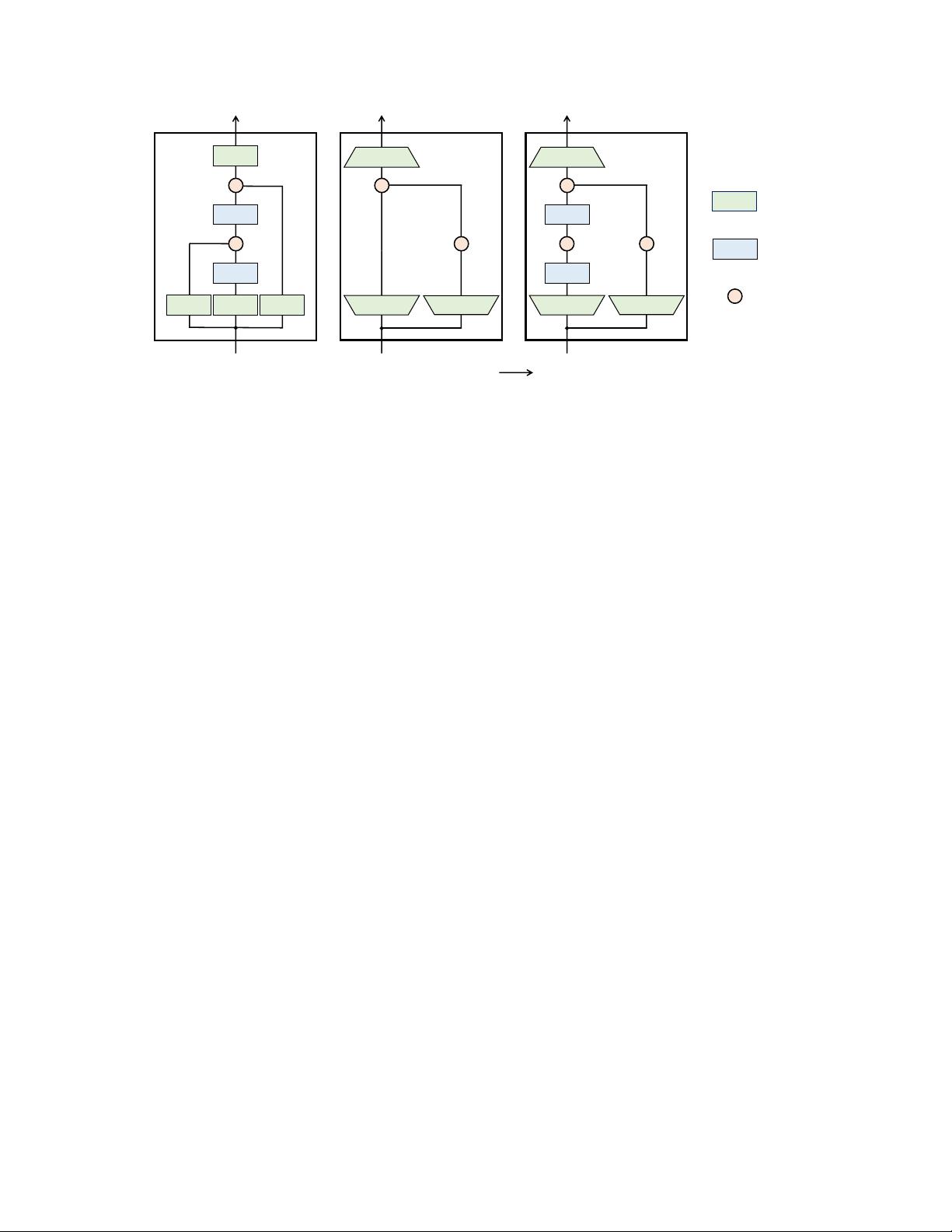
3.4 A Simplied SSM Architecture

As with structured SSMs, selective SSMs are standalone sequence transformations that can be ﬂexibly incorporated

into neural networks. The H3 architecture is the basis for the most well-known SSM architectures (Section 2), which

are generally comprised of a block inspired by linear attention interleaved with an MLP (multi-layer perceptron)

block. We simplify this architecture by combining these two components into one, which is stacked homogenously

(Figure 3). This is inspired by the gated attention unit (GAU) (Hua et al. 2022), which did something similar for

attention.

This architecture involves expanding the model dimension

𝐷

by a controllable expansion factor

𝐸

. For each

block, most of the parameters (

3𝐸𝐷

) are in the linear projections (

2𝐸𝐷

for input projections,

𝐸𝐷

for output

projection) while the inner SSM contributes less. The number of SSM parameters (projections for

∆, B, C

, and

H3 Gated MLP

Mamba

Linear

projection

Sequence

transformation

Nonlinearity

(activation or

multiplication)

XX X

Conv

SSM

Conv

SSM

⨂

Figure 3: (Architecture.) Our simplied block design combines the H3 block, which is the basis of most SSM architectures, with

the ubiquitous MLP block of modern neural networks. Instead of interleaving these two blocks, we simply repeat the Mamba block

homogenously. Compared to the H3 block, Mamba replaces the rst multiplicative gate with an activation function. Compared to

the MLP block, Mamba adds an SSM to the main branch. For 𝜎 we use the SiLU / Swish activation (Hendrycks and Gimpel 2016;

Ramachandran, Zoph, and Quoc V Le 2017).

the matrix

) are much smaller in comparison. We repeat this block, interleaved with standard normalization

and residual connections, to form the Mamba architecture. We always ﬁx to

𝐸 = 2

in our experiments and use two

stacks of the block to match the

12𝐷

parameters of a Transformer’s interleaved MHA (multi-head attention) and

MLP blocks. We use the SiLU / Swish activation function (Hendrycks and Gimpel 2016; Ramachandran, Zoph,

and Quoc V Le 2017), motivated so that the Gated MLP becomes the popular “SwiGLU” variant (Chowdhery

et al. 2023; Shazeer 2020; Touvron et al. 2023). Finally, we additionally use an optional normalization layer (we

choose LayerNorm (J. L. Ba, Kiros, and Hinton 2016)), motivated by RetNet’s usage of a normalization layer in a

similar lo cation (Y. Sun et al. 2023).

3.5 Properties of Selection Mechanisms

The selection mechanism is a broader concept that can be applied in diﬀerent ways, such as to more traditional

RNNs or CNNs, to diﬀerent parameters (e.g.

in Algorithm 2), or using diﬀerent transformations

𝑠(𝑥)

3.5.1 Connection to Gating Mechanisms

We highlight the most important connection: the classical gating mechanism of RNNs is an instance of our selection

mechanism for SSMs. We note that the connection between RNN gating and the discretization of continuous-time

systems is well established (Funahashi and Nakamura 1993; Tallec and Ollivier 2018). In fact, Theorem 1 is

an improvement of Gu, Johnson, Goel, et al. (2021, Lemma 3.1) generalizing to the ZOH discretization and

input-dependent gates (proof in Appendix C). More broadly,

∆

in SSMs can be seen to play a generalized role

of the RNN gating mechanism. In line with prior work, we adopt the view that discretization of SSMs is the

principled foundation of heuristic gating mechanisms.

Theorem 1. When 𝑁 = 1, A = −1, B = 1, 𝑠

∆

= 𝖫𝗂𝗇𝖾𝖺𝗋(𝑥), and 𝜏

∆

= 𝗌𝗈𝖿𝗍𝗉𝗅𝗎𝗌, then the selective SSM recurrence

(Algorithm 2) takes the form

𝑔

𝑡

= 𝜎(𝖫𝗂𝗇𝖾𝖺𝗋(𝑥

𝑡

))

ℎ

𝑡

= (1 − 𝑔

𝑡

)ℎ

𝑡−1

+ 𝑔

𝑡

𝑥

𝑡

(5)

As mentioned in Section 3.2, our speciﬁc choices of

𝑠

∆

, 𝜏

∆

is from this connection. In particular, note that if a

given input

𝑥

𝑡

should be completely ignored (as necessary in the synthetic tasks), all

𝐷

channels should ignore it,

and so we project the input down to 1 dimension before repeating/broadcasting with ∆.

剩余36页未读，继续阅读

CS-Polaris

粉丝: 958
资源: 8

Mamba：线性时间序列建模与选择性状态空间

Linear models.pdf

SCALE-MAMBA:SCALE-MAMBA MPC系统的存储库

mamba-ssm-1.2.0.post1-py3-none-any.whl

mamba-ssm-1.1.3-py3-none-any.whl

Python库 | akc_mamba-2.1.0-py3-none-any.whl

pos-mamba-sdk-develop-源码.rar

Python库 | akc-mamba-2.1.0a2.tar.gz

libuuid-devel-2.25-2mamba.i586.rpm

3DMGAME-NBA.2K21.Mamba.Forever.Edition-3DM.torrent

Mamba selective-scan-cuda-linux-gnu.so

最新资源