JOURNAL OF L
A
T
E
X CLASS FILES, VOL. XX, NO. XX, AUGUST 2019 5
Grap h
𝑋
𝑅𝑒𝐿𝑢 𝑅𝑒𝐿𝑢
Outputs
Gconv
…
Gconv
…
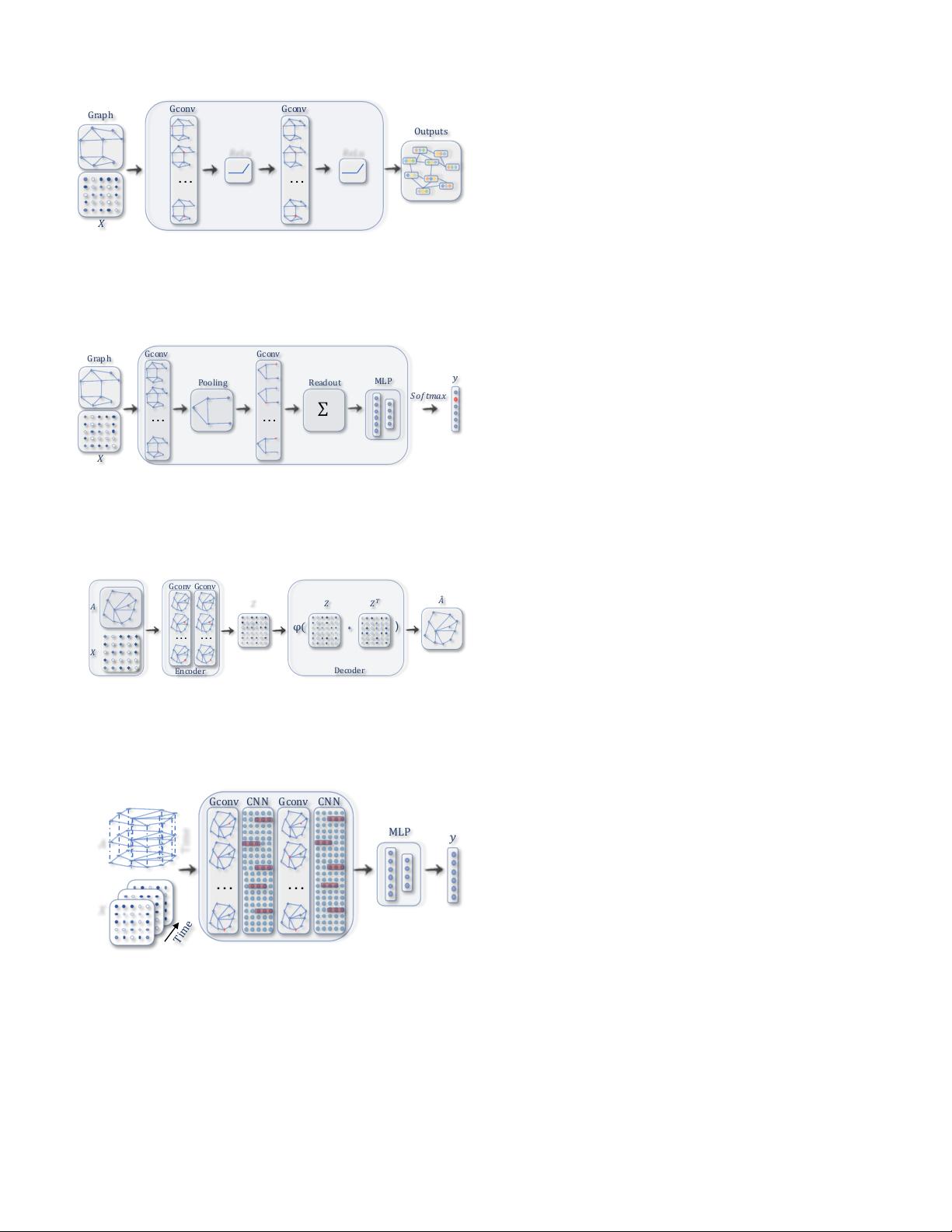
(a) A ConvGNN with multiple graph convolutional layers. A graph convo-
lutional layer encapsulates each node’s hidden representation by aggregating
feature information from its neighbors. After feature aggregation, a non-linear
transformation is applied to the resulted outputs. By stacking multiple layers,
the final hidden representation of each node receives messages from a further
neighborhood.
Gconv
Grap h
Readout
Gconv
Pooling
𝑆𝑜𝑓𝑡𝑚𝑎𝑥
𝑋
… …
MLP
𝑦
∑
(b) A ConvGNN with pooling and readout layers for graph classification
[21]. A graph convolutional layer is followed by a pooling layer to coarsen
a graph into sub-graphs so that node representations on coarsened graphs
represent higher graph-level representations. A readout layer summarizes the
final graph representation by taking the sum/mean of hidden representations
of sub-graphs.
𝑍"
φ(
𝑍
%
𝑍
∗
)
𝐴
𝑋
𝐴
)
Decode r
Encoder
…
Gconv"Gconv
…
(c) A GAE for network embedding [61]. The encoder uses graph convolutional
layers to get a network embedding for each node. The decoder computes the
pair-wise distance given network embeddings. After applying a non-linear
activation function, the decoder reconstructs the graph adjacency matrix. The
network is trained by minimizing the discrepancy between the real adjacency
matrix and the reconstructed adjacency matrix.
𝐴
𝑋
Time
'''Gconv'''CNN''''Gconv ''''CNN
… …
MLP
𝑦
Time
(d) A STGNN for spatial-temporal graph forecasting [74]. A graph convolu-
tional layer is followed by a 1D-CNN layer. The graph convolutional layer
operates on A and X
(t)
to capture the spatial dependency, while the 1D-CNN
layer slides over X along the time axis to capture the temporal dependency.
The output layer is a linear transformation, generating a prediction for each
node, such as its future value at the next time step.
Fig. 2: Different Graph Neural Network Models built with
graph convolutional layers. The term Gconv denotes a graph
convolutional layer (e.g., GCN [22]). The term MLP denotes
multilayer perceptrons. The term CNN denotes a standard
convolutional layer.
latent representation upon which a decoder is used to re-
construct the graph structure [61], [62]. Another popular
way is to utilize the negative sampling approach which
samples a portion of node pairs as negative pairs while
existing node pairs with links in the graphs are positive
pairs. Then a logistic regression layer is applied after the
convolutional layers for end-to-end learning [42].
In Table III, we summarize the main characteristics of
representative RecGNNs and ConvGNNs. Input sources, pool-
ing layers, readout layers, and time complexity are compared
among various models.
IV. RECURRENT GRAPH NEURAL NETWORKS
Recurrent graph neural networks (RecGNNs) are mostly pi-
oneer works of GNNs. They apply the same set of parameters
recurrently over nodes in a graph to extract high-level node
representations. Constrained by computation power, earlier
research mainly focused on directed acyclic graphs [13], [80].
Graph Neural Network (GNN*
2
) proposed by Scarselli et
al. extends prior recurrent models to handle general types of
graphs, e.g., acyclic, cyclic, directed, and undirected graphs
[15]. Based on an information diffusion mechanism, GNN*
updates nodes’ states by exchanging neighborhood information
recurrently until a stable equilibrium is reached. A node’s
hidden state is recurrently updated by
h
(t)
v
=
X
u∈N(v)
f(x
v
, x
e
(v,u)
, x
u
, h
(t−1)
u
), (1)
where f(·) is a parametric function, and h
(0)
v
is initialized
randomly. The sum operation enables GNN* to be applicable
to all nodes, even if the number of neighbors differs and no
neighborhood ordering is known. To ensure convergence, the
recurrent function f(·) must be a contraction mapping, which
shrinks the distance between two points after mapping. In the
case of f(·) being a neural network, a penalty term has to
be imposed on the Jacobian matrix of parameters. When a
convergence criterion is satisfied, the last step node hidden
states are forwarded to a readout layer. GNN* alternates the
stage of node state propagation and the stage of parameter
gradient computation to minimize a training objective. This
strategy enables GNN* to handle cyclic graphs. In follow-up
works, Graph Echo State Network (GraphESN) [16] extends
echo state networks to improve efficiency. GraphESN consists
of an encoder and an output layer. The encoder is randomly
initialized and requires no training. It implements a contractive
state transition function to recurrently update node states until
the global graph state reaches convergence. Afterward, the
output layer is trained by taking the fixed node states as inputs.
Gated Graph Neural Network (GGNN) [17] employs a gated
recurrent unit (GRU) [81] as a recurrent function, reducing the
recurrence to a fixed number of steps. The advantage is that it
no longer needs to constrain parameters to ensure convergence.
2
As GNN is used to represent broad graph neural networks in the survey,
we name this particular method GNN* to avoid ambiguity.


