水下机器人单目SLAM算法实现与评估

需积分: 50 66 浏览量更新于2024-07-18 5 收藏 36.79MB PDF 举报

"这篇硕士论文主要探讨了水下机器人单目SLAM（Simultaneous Localization and Mapping，同时定位与建图）的实现与评估。作者Chris Kahlefendt在论文中详细介绍了SLAM的基本概念、数学模型、不同类型的SLAM算法，并特别关注了水下环境下的SLAM挑战和解决方案。此外，还对ORBSLAM算法进行了深入的研究，包括特征提取、数据关联、初始化和跟踪等关键步骤。" SLAM是机器人技术中的一个重要领域，它允许机器人在未知环境中构建地图的同时进行自我定位。在水下环境，由于光线散射、能见度低以及传感器性能受限，SLAM的实现变得更加复杂和具有挑战性。论文首先介绍了SLAM的基本原理，包括数学模型的建立。SLAM问题通常通过滤波器（如EKF-SLAM）或图优化（如GraphSLAM）的方法来解决。EKF-SLAM使用扩展卡尔曼滤波进行状态估计，而GraphSLAM则将SLAM问题表示为一个优化问题，通过最小化误差图来找到最佳估计。接着，论文讨论了多种具体的SLAM实现，例如： 1. FastSLAM：这是一种粒子滤波器方法，用于实时地估计机器人轨迹和地图。 2. DTAM（ Dense Tracking and Mapping）：该算法实现了稠密的实时三维重建和运动估计。 3. RatSLAM：受老鼠导航启发，适用于资源有限的机器人系统。 4. ORBSLAM：这是一种基于特征的SLAM系统，使用ORB（Oriented FAST and Rotated BRIEF）特征进行跟踪和地图构建，具有高效和鲁棒性。 5. LSDSLAM（Large-Scale Direct Monocular SLAM）：侧重于大规模场景的直接法SLAM，无需预先计算特征点，而是直接处理图像像素。在水下环境下，SLAM面临更多独特挑战，如光学畸变、水下目标的模糊以及水体的动态特性等。论文中提到了现有的一些水下SLAM方法，但同时也指出这些方法的局限性，并分析了这些挑战如何影响SLAM的性能。最后，作者选择了ORBSLAM作为水下机器人的SLAM算法，详细分析了其工作流程，包括特征提取（如ORB特征检测）、数据关联（确保新观测到的特征与已知地图点匹配）、初始化（建立初始位姿估计）和跟踪（持续更新机器人位置并维护地图的完整性）等步骤。这篇论文全面地探讨了水下环境中的SLAM问题，提供了对不同SLAM算法的理解，并且对ORBSLAM在水下应用中的潜力进行了深入研究，对于水下机器人技术和SLAM算法的发展具有重要的参考价值。

8 2.2 Example Implementations

In EKF-SLAM the motion model is modelled as:

P (x

k−1

, u

) ⇐⇒ x

= f(x

k−1

, u

) + w

(2.6)

and the observation model as:

P (z

, m) ⇐⇒ z

= h(x

, m) + v

(2.7)

where

and

resemble zero-mean, white Gaussian noise,

models the robot’s kinematics

and

describes the geometry of the observation [6]. The added noise values are used to

deal with the uncertainty in the measurements.

Implementing an EKF back-end comes with a couple of problems as pointed out by [5] and

[6]. First, the computational costs rise quadratically with the amount of landmarks kept

in the map [9]. This leads to problems when wanting to create feature rich or large maps.

This can however be reduced to a linear relationship as explained in [10]. Second, due to

the assumption that

and

are zero-mean, white and Gaussian the linearization used in

the EKF can cause intolerable errors in the estimation. Third, the EKF cannot incorporate

negative observations

in its estimations due to its Gaussian nature. Consequently it does

not process all available information.

Even though EKF-SLAM has these limitations EKFs are a widely used back-end and can

be regarded as a well researched topic that can achieve very good results when used under

the right conditions.

2.2.2 FastSLAM

The idea of FastSLAM was ﬁrst introduced by Montemerlo et al. [11] in 2002. This section

will explain what is known as FastSLAM2.0, since this implementation has been proven to

be superior [12]. What makes FastSLAM possible is a structural property of the SLAM

problem: “correlations in the uncertainty among diﬀerent map features [landmark position

estimates] arise only through robot pose uncertainty” [13]. Thanks to this, the problem

can be split into two subproblems. First: the robot localization which is done with the

help of particle ﬁlters

in FastSLAM. Second: estimating the landmark locations. In order

to be able to split the SLAM problem into these two parts the assumption has to be made

that the exact robot pose history is known.

Doing this the SLAM problem 2.1 can be rewritten as:

P (X

0:k

, m|Z

0:k

, U

0:k

, x

) = P (m|X

0:k

, Z

0:k

)P (X

0:k

, U

0:k

, x

) (2.8)

0:k

= {x

, x

, ..., x

} : Robot pose history

The absence of a landmark that is expected to be there.

A probabilistic approach to solving the localization problem. Each particle represents a hypothesis for

the current robot location. Over time, given enough data, particles in wrong locations are removed

while those that are most likely to be correct remain. An explanation is given in [14].

2 Simultaneous Localization and Mapping (SLAM) 9

Note that this is now the probability distribution on the pose history

0:k

rather than

the single pose

. In FastSLAM each particle computes an estimate of the robot’s pose

based on its individual pose and measurement history. These estimates are then given

weights which decay over time. In a resampling step old erroneous particles are replaced

with new ones when necessary. At which time to resample best is an open problem [6].

As can be seen in equation 2.8 the landmark estimation

(

m|X

0:k

, Z

0:k

) depends on the

pose history

0:k

which is bound to a single particle. Therefore each particle requires its

own landmark location estimation. Another feature of FastSLAM is that estimating the

landmark’s positions can be done for each landmark individually. This is generally done

using one EKF per landmark. While this sounds like it would increase the computational

costs as compared to EKF-SLAM, it does in fact potentially decrease them. Since the

matrices used by the EKFs stay much smaller the computation cost can be reduced to

(

Nlog

(

)) with

being the number of landmarks and N the number of particles used.

A detailed overview over the diﬀerences between FastSLAM and EKF-SLAM can be found

in the work of Calonder [15].

Just like EKF-SLAM, FastSLAM only proposes a back-end and can be used with diﬀerent

front-ends. An interesting factor about FastSLAM is that, due to the nature of the particle

ﬁlter, each particle can implement its own front-end.

2.2.3 Graph SLAM

Graph SLAM is a variant of SLAM which does not run and update while the robot is

moving and collecting data. It is what is considered to be an oﬄine SLAM approach

which solves the so-called full SLAM problem [16]. For the full SLAM problem the full

pose history

0:k

and the map

are calculated from the full set of measurements

0:k

and control inputs

0:k

. The advantage of this approach is that instead of processing

and then discarding the measurement data like in ﬁltering approaches (e.g. EKF-SLAM

and FastSLAM), the data is recorded and then used at the time of map building. This

generally achieves higher map accuracy than the ﬁltering techniques [17].

In Graph SLAM the SLAM problem is considered in its graph-based formulation where

each node represents a robot pose or a landmark observation and the edges symbolize

sensor measurements that constrain the measured poses and landmark observations. An

example for a resulting graph is presented in ﬁgure 2.4.

The constraints represented by the edges of the graph are generally of nonlinear nature.

Graph SLAM resolves these by linearizing them and applying standard optimization

techniques. This way it is possible to ﬁnd the conﬁguration of robot poses that best ﬁts

the underlying constraints. A mathematical derivation and detailed explanations about

the used algorithms can be found in [17].

Summarizing Graph SLAM can be regarded as split into two parts: constructing a graph

from data readings and optimizing this graph to ﬁnd the most likely conﬁguration of robot

poses given the introduced constraints. Generally the ﬁrst part is handled by the front-end

which needs to be deﬁned in such a way that it forms a graph from its observations. The

second part is handled by the back-end which performs the graph optimization. The actual

2 Simultaneous Localization and Mapping (SLAM) 11

2.2.4 DTAM

DTAM is a monocular SLAM approach which is capable of creating dense 3D models from

a single moving camera [19]. It does this by using a depth map which is created from

multiple frames with diﬀerent viewpoints of the same scenery. One such created model is

shown in ﬁgure 2.6.

(a) (b) (c) (d)

(e)

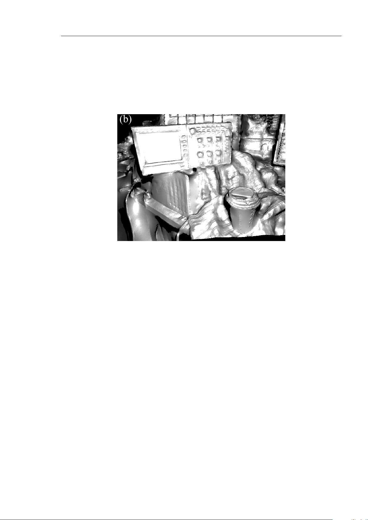
Figure 5. Example inverse depth map reconstructions obtained from DTAM using a single low sample cost volume with S = 32. (a)

Regularised solution obtained without the sub-sample reﬁnement is shown as a 3D mesh model with Phong shading (inverse depth map

solution shown in inset). (b) Regularised solution with sub-sample reﬁnement using the same cost volume also shown as a 3D mesh model.

(c) The video frame as used in PTAM, with the point model projections of features found in the current frame and used in tracking. (d,e)

Novel wide baseline texture mapped views of the reconstructed scene used for tracking in DTAM.

The reﬁnement step is embedded in the iterative optimisa-

tion scheme by replacing the located a

n+1

with the sub-

sample accurate version. It is not possible to perform this

reﬁnement post-optimisation, as at that point the quadratic

coupling energy is large (due to a very small θ), and so

the ﬁtted parabola is a spike situated at the minimum. As

demonstrated in Figure 5 embedding the reﬁnement step in-

side each iteration results in vastly increased reconstruction

quality, and enables detailed reconstructions even for low

sample rates, e.g. S ≤ 64.

2.2.6 Setting Parameter Values and Post Processing

Gradient ascent/descent time-steps σ

, σ

are set optimally

for the update scheme provided as detailed in [3]. Various

values of β can be used to drive θ towards 0 as iterations in-

crease while ensuring θ

n+1

< θ

(1 − βn). Larger values

result in lower quality reconstructions, while smaller values

of β with increased iterations result in higher quality. In our

experiments we have set β = 0.001 while θ

≥ 0.001 else

β = 0.0001 resulting in a faster initial convergence. We

use θ

= 0.2 and θ

end

= 1.0e − 4. λ should reﬂect the

data term quality and is set dynamically to 1/(1 + 0.5

d),

where

d is the minimum scene depth predicted by the cur-

rent scene model. For the ﬁrst key-frame we set λ = 1. This

dynamically altered data term weighting sensibly increases

regularisation power for more distant scene reconstructions

that, assuming similar camera motions for both closer and

further scenes, will have a poorer quality data term.

Finally, we note that optimisation iterations can be inter-

leaved with updating the cost volume average, enabling the

surface (though in a non fully converged state) to be made

available for use in tracking after only a single ρ computa-

tion. For use in tracking, we compute a triangle mesh from

the inverse depth map, culling oblique edges as described in

[9].

2.3. Dense Tracking

Given a dense model consisting of one or more keyframes,

we can synthesise realistic novel views over wide baselines

by projecting the entire model into a virtual camera. Since

such a model is maintained live, we beneﬁt from a fully pre-

dictive surface representation, handling occluded regions

and back faces naturally. We estimate the pose of a live

camera by ﬁnding the parameters of motion which generate

a synthetic view which best matches the live video image.

We reﬁne the live camera pose in two stages; ﬁrst with

a constrained inter-frame rotation estimation, and second

with an accurate 6DOF full pose reﬁnement against the

model. Both are formulated as iterative Lucas-Kanade style

non-linear least-squares problems, iteratively minimising

an every-pixel photometric cost function. To converge to

the global minimum, we must initialise the system within

the convex basin of the true solution. We use a coarse-ﬁne

strategy over a power of two image pyramid for efﬁciency

and to increase our range of convergence.

2.3.1 Pose Estimation

We ﬁrst follow the alignment method of [8] between con-

secutive frames to obtain rotational odometry at lower levels

within the pyramid, offering resilience to motion blur since

consecutive images are similarly blurred. This optimisa-

tion is more stable than 6DOF estimation when the number

of pixels considered is low, helping to converge for large

pixel motions, even when the true rotation is not strictly ro-

tational (Figure 6). A similar step is performed before fea-

ture matching in PTAM’s tracker, computing ﬁrst the inter-

frame 2D image transform and ﬁtting a 3D rotation [7].

The rotation estimate helps inform our current best estimate

of the live camera pose,

. We project the dense model

in to a virtual camera v at location T

, with colour

Figure 2.6: An example of an environment modelled with DTAM. Figure source: [19]

The camera movement is then tracked by aligning the whole image with the textured 3D

model. According to Newcombe et al.[19] tracking works in real time and supersedes other

approaches like Parallel Tracking and Mapping (PTAM) [20], especially when the camera

is moved quickly and looses focus.

As this approach works with large images on a per pixel basis it is very computationally

expensive and heavily relies on Graphics Processing Unit (GPU)-based parallel computation.

Newcombe et al. also mention that the algorithm has problems with tracking in dynamic

lighting conditions.

剩余126页未读，继续阅读

ab1233123

粉丝: 4
资源: 5

水下机器人单目SLAM算法实现与评估

dolphin_slam:解决水下环境中SLAM问题的仿生方法

0861-极智开发-解读求解模线性方程及示例代码

matlab的slam代码-uwimageproc:基于OpenCV的水下视频和图像处理工具箱

激光移动机器人高精度SLAM算法与实现1

"室内机器人单目视觉SLAM算法研究-高智能化移动机器人的关键技术

单目视觉移动机器人SLAM系统设计与实现

在水下机器人应用中，ORBSLAM算法如何处理单目视觉SLAM中的尺度不确定性问题？

单目机器人SLAM算法研究

室内机器人的单目视觉SLAM算法研究1

"激光移动机器人高精度SLAM算法与实现研究

最新资源