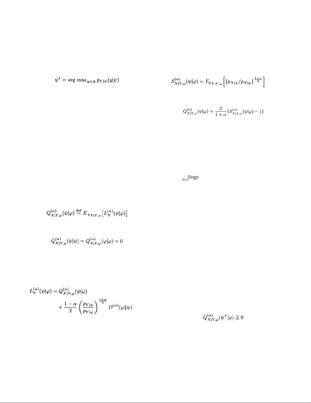
In the D-EM algorithm, the above likelihood ratios are
always used instead of logarithmic likelihood.
3.2. Maximization of incomplete-data
likelihood
The model which best explains the appearance of the
observable data y satisfies
Here, < is a Euclidean space or its subset which has the
same dimension as \ and M. This maximization is equiva-
lent to that of the incomplete-data D-log likelihood ratio.
The D-EM algorithm given in the next section is a method
for performing this maximization by using the conditional
expectation of the complete-data D-log likelihood ratio. In
the case of D = 1, this maximization is reduced to that of
log-likelihood. This is the traditional EM algorithm. In this
paper, therefore, it is often referred to the log-EM algo-
rithm.
4. The D-EM Algorithm and Its Family
4.1. Basic equality for the
D
-EM algorithm
First, we define the expectation of the complete-data
D-log likelihood ratio conditioned by the observed data:
This Q
D
-function has the following property:
Next, we compute the D-divergence between two condi-
tional probability densities p
X
|
Y
,
\
x
|
y, \ and p
X
|
Y
,
M
x|y, M
by using Eq. (1). After mathematical computation using the
Bayes formula, the following equation is obtained. This is
the basic equality for the D-EM algorithm:
It is important to observe that the second term on the
right-hand side is nonnegative for D < 1. Therefore, the
incomplete-data D-log likelihood ratio of the left-hand side
is always nonnegative if the Q
D
-function of the right-hand
side is kept nonnegative on the update of M. Then, the D-EM
algorithm is obtained as follows.
[D-EM algorithm I]
[E-step] Compute (9) analytically. In the case of D =
1, the computation is performed using the logarithm.
[M-step] For D < 1, obtain \
<
which maximizes
(9).
[U-step] Check to see if the algorithm is converged.
If not, then replace
M
by
\
*
and go back to the E-step.
Next, we extract the core part of the Q
D
-function as
Since there is a relationship
the
D
-EM algorithm is classified into the following cases.
[
D
-EM algorithm II]
[E-step] Compute (11) mathematically. In the case of
D
= 1, the usual logarithm is used.
[M-step]
(i) For the case of
1
D
1
, compute
\
which
maximizes (11).
(ii) For the case of
D
= 1, compute
\
which maxi-
mizes E
p
X
|
Y
,
M
[logp
X
|
\
]
.
(iii) For the case of
D
< 1, compute
\
which
minimizes (11).
[U-step] Check to see if the algorithm is converged.
If not, then replace
M
by
\
and go back to the E-step.
The convergence properties of the
D
-EM algorithm
are discussed in the next section together with generalized
algorithms.
4.2. The D-GEM algorithm
Dempster and colleagues [1] presented the GEM
algorithm (Generalized EM algorithm) which uses incre-
mental updates possibly weaker than the maximization per
se. Such a GEM algorithm is important for the case that
exact arg max cannot be obtained analytically. The D-
GEM algorithm using the D-log likelihood ratio is de-
scribed as follows:
[D-GEM algorithm]
[M-step] For D < 1, compute the update value
\
< such that
Since the D-EM algorithm satisfies (12), it is a special
case of the D-GEM algorithm. On the convergence of the
D-GEM algorithm, we have two theorems. Theorem 1
states the convergence of the incomplete-data D-log likeli-
(9)
(10)
(11)
(12)
14


