systems and switched arrival systems are some of the
generalized models [23–27]. A more detailed description of
such applications could be found in Morse [28].
The stability of a switched system is a basic problem,
which is affected by two factors: the stability of its
subsystems and the switching rule. The supply chain
syste m investigated in this paper is considered as an
autonomous switched system, and its stability analysis is
decomposed into three parts: analysis of the dynamics of
the linear subsystems, analysis of switching rules, and
analysis of the stability of supply chain under the switching
rules. This analys is method can more easily handle the
stability and dynamics of the system than using t he
nonlinear system theory.
3 Basic dynamic model
3.1 System description
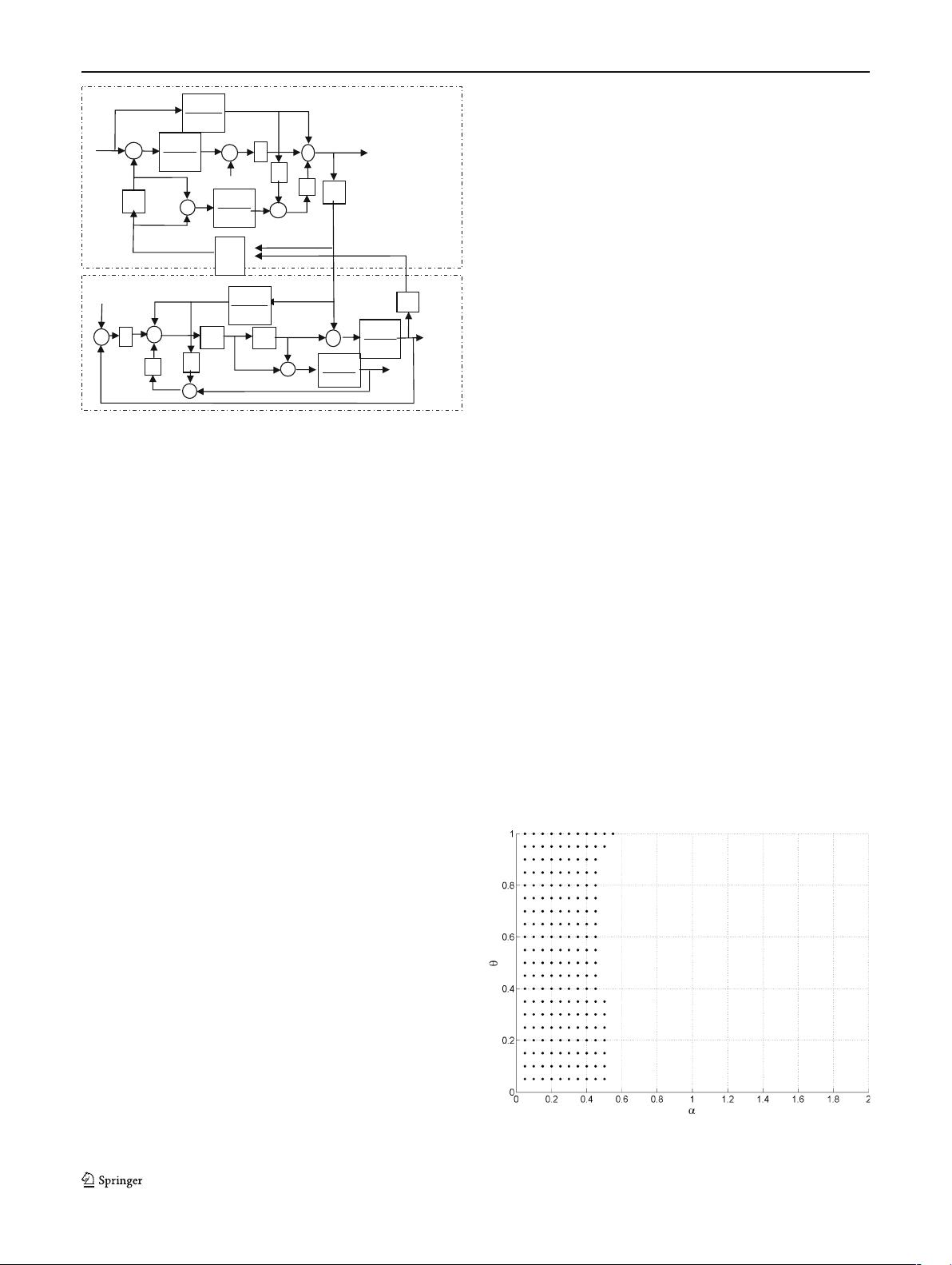
The system under study is a typical cascaded production–
distribution system consisting of two secto rs: a retailer and
a distributor (see Fig. 1 ). Customer demand is exogenous.
Given that stocks are available, each sector must supply the
amount requested by the next sector. If the stocks are
insufficient, surplus orders must be kept in backlog until
deliveries can be made. With the assumption that the
system is a periodic-reviewed supply chain, the sequenc e of
events during a period is, first, the member observes and
satisfies consumer demand if there is no backlog and then
receives goods; next, the member observes the new
inventory level and finally places an order on its supplier.
Based on this arrangement, there is a period from the time
the order is sent until the supplier receives it. Suppose it
takes the distributor l periods to transport goods to the
retailer. The total lead time is then given by L=l+1. To
simplify the model without loss of generality, we assume
that the outside supplier’s lead time is L as well. It is
assumed that the outside supplier has infinite inventory so
that the distributor’s order can be fully satisfied. Cap acity
of the distributor is assumed to be limited. Therefore, he
will satisfy the retailer’s demand based on his inventory
level.
3.2 Block diagram and difference equations of the system
Model notation Hereafter, let r, d,ands denote t he
retailer’s state variables, the distributor’s state variables,
and the outside supplier’s state variables, respectively.
t time period, t=1,2,...;
D(t) the outside demand at time period t
I
i
(t) inventory level of member i at the end of time
period t, i∈ {r,d}, and similarly below
BL
i
(t) backup orders of member i at the end of time
period t
O
i
(t) order quantity of member i at the end of time
period t
R
i
(t) quantity of goods that member i received at the
beginning of time period t
S
i
(t) shipments of mem ber i to its downstream
member at time period t
S
s
(t) shipments of outside supplier to the distributor at
time period t
WIP
i
(t) work in progress of member i at time period t
F
i
(t) forecasted demand of member i in period t
)(tD
)(tO
r
1
Z
l
l
1
α
)(tS
d
1
1
1
z
1
1
1
z
0
r
I
β
1
1
1
1
z
1
1
1
z
)(tI
r
)(tWIP
r
+
+
+
+
+
+
+
-
-
-
-
-
-
-
-
+
+
+
+
+
+
+
0
d
I
L
1
1
1
z
θ
1
1
1
z
)(tWIP
d
)(tI
d
)(tO
d
)(tF
d
)(tF
r
Distributor
Retailer
)(t
σ
_
_
_
_
_
_
_
_
_
_
θ
_
_
_
_
_
_
_
_
_
θ
θ
β
α
Fig. 2 The block diagram of the supply chain
Fig. 3 The states of the eigenvalues of subsystem 15
202 Int J Adv Manuf Technol (2009) 43:200–210


