matching process, viz. avoid comparing all records from one source with all records coming from another source. Indexing the data
produces data structures that facilitate an effective generation of candidate record pairs, which likely are matches, or may refer to the
same entity.
At the second step, the record pair comparison analysis starts, where candidate record pairs from the indexed data structures are
compared by using various (selected) field comparison functions (methods). Once all the results or scores have been obtained, at the
third step, the comparison scores are split into training and testing sets. The idea behind this step is to adjust (train) the learning
structure (algorithm) with the training set, and then present new unseen record pairs to the decision model generated to assess its
performance. The known outputs (matches or non-matches) coming from the training set are used as a target to carry out supervised
learning. Subsequently, the training of the algorithm starts. Afterwards, the training set is fed to the network, and the error is
evaluated and back propagated into the model until a desired output is achieved or a number of iterations is completed. The final
step is the performance assessment of the model; here we determine how many matches, non-matches, and potential matches (“?”)
were classified. If record pairs are classified as “?”, these will require a clerical review. We also need to count the number of false
positives and false negatives and review these records to find out why they were misclassified.
3.1. The development of the learning model
Now that we have a better grasp of the overall process, we detail the construction of the decision models in the following sections
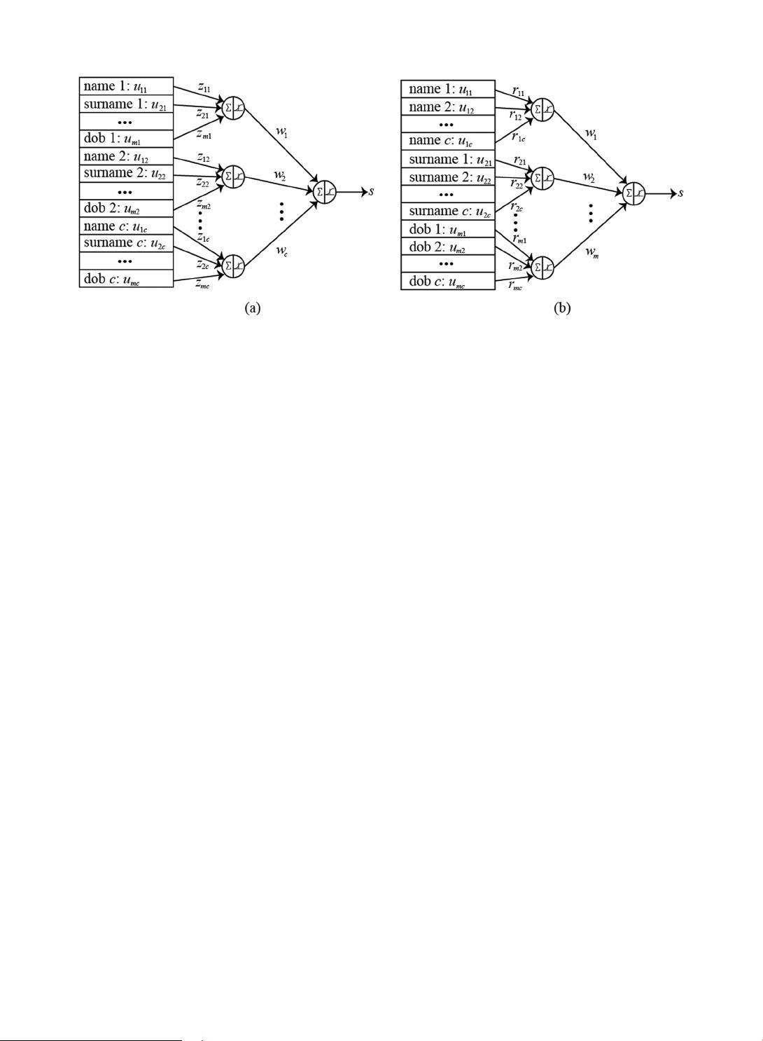
(see Figs. 2(a) and 2(b)). Since the proposed models heavily rely on the learning algorithm, we will concentrate on the fourth step. To
offer a better explanation, and to maintain conciseness of the presentation, let us consider that the decision model is constructed on
the basis of experimental data, which in most cases come as a collection of input-output data pairs
uktk((),())
ij
, k =1,2,…, N; i =1,2,
…, m; j =1,2,…, c, where u(k)
R
mc
and t(k)
R. More specifically, u(k)
[0, 1]
mc
and t(k)
[0, 1], where N is the number of
record pairs compared, m is the number of data fields selected, c is the number of comparison functions, and
m
is the size of each
vector u, which corresponds to all m fields processed by each j
th
method. The j
th
method applied to the i
th
field returns a matching
result u
ij
. To aggregate these results, two architectures (models) are considered. In both figures, for illustration purposes, let us
assume that field 1 corresponds to the name, field 2 to surname, and field m to DOB, and each field is processed by j =1,2,…, c
comparison methods. The way the fields are aggregated is di fferent in each model, as illustrated in Fig. 2.
Once all the scores have been produced, at the third step and the data are split into training and testing sets, an aggregation of the
scores starts. For Model 1 (Fig. 2(a)), each jth node only aggregates the fields where the jth comparison function was used, and there
are no other weights connecting with nodes corresponding to the other j +1,j +2,…, j + c – 1 functions. Considering all m fields
coming from the training set, and only the jth comparison function, the aggregate result y
j
is,
∑
uz y fp=,=(
j
i
m
ij ij
jj
=1
(1)
where f is a monotonically increasing function with values in (0, 1). z is a vector of weights z =
zz z
,, …,
jj mj12
initially with values in
[−1, 1], which expresses the significance of the i=1, 2, …, m fields. Considering all y
j
, j =1,2,…, c aggregations, we obtain the final
aggregated score s in the following form,
∑
lywsfl=,=(
j
c
j
j
=1
(2)
where w =[
ww,, …,
12
] is a second vector of weights which expresses the relevance of each function, and s is the output of the
Fig. 2. Aggregation of the scores coming from (a) different comparison methods or (b) different fields. Here each node sums the inputs multiplied by a weight and
then a sigmoid activation function computes the result of the aggregation for each node.
O.F. Reyes-Galaviz et al.
Data & Knowledge Engineering 112 (2017) 106–129
110


