deconvolution, and unpooling. U-Net [43] combines skip
layers and learned deconvolution for pixel labeling of
microscopy images. The dilation architecture of [44] makes
thorough use of dilated convolution for pixel-precise output
without a random field or skip layers.
3FULLY CONVOLUTIONAL NETWORKS
Each layer output in a convnet is a three-dimensional
array of size h w d,whereh and w are spatial dimen-
sions, and d is the feature or channel dimension. The first
layer is the image, with pixel size h w,andd cha nnels.
Locations in higher layers correspond to the locations in
the image they are p ath-con nected to, which are called
their receptive fields.
Convnets are inherently translation invariant. Their basic
components (convolution, pooling, and activation func-
tions) operate on local input regions, and depend only on
relative spatial coordinates. Writing x
ij
for the data vector at
location ði; jÞ in a particular layer, and y
ij
for the following
layer, these functions compute outputs y
ij
by
y
ij
¼ f
ks
fx
siþdi;sjþdj
g
0di;dj<k
;
where k is called the kernel size, s is the stride or subsam-
pling factor, and f
ks
determines the layer type: a matrix
multiplication for convolution or average pooling, a spatial
max for max pooling, or an elementwise nonlinearity for an
activation function, and so on for other types of layers.
This functional form is maintained under composition,
with kernel size and stride obeying the transformation rule
f
ks
g
k
0
s
0
¼ðf gÞ
k
0
þðk1Þs
0
;ss
0
:
While a general net computes a general nonlinear function,
a net with only layers of this form computes a nonlinear fil-
ter, which we call a deep filter or fully convolutional network.
An FCN naturally operates on an input of any size, and pro-
duces an output of corresponding (possibly resampled) spa-
tial dimensions.
A real-valued loss function composed with an FCN
defines a task. If the loss function is a sum over the spatial
dimensions of the final layer, ‘ðx; uÞ¼
P
ij
‘
0
ðx
ij
; uÞ, its
parameter gradient will be a sum over the parameter gra-
dients of each of its spatial components. Thus stochastic gra-
dient descent on ‘ computed on whole images will be the
same as stochastic gradient descent on ‘
0
, taking all of the
final layer receptive fields as a minibatch.
When these receptive fields overlap significantly, both
feedforward computation and backpropagation are much
more efficient when computed layer-by-layer over an entire
image instead of independently patch-by-patch.
We next explain how to convert c lassification nets into
fully c onvolutional nets that produce coarse output maps.
For pixelwise prediction, we need to connect these coarse
outputs back to the pixels. Section 3.2 describes a trick
used for this purpose (e.g., by “fast scannin g” [45]). We
explain this trick in terms of network modification. As an
efficient, effective alternative, we upsample in Section 3.3,
reusing our impl eme ntatio n of convol ution. In Se cti on 3.4
we con sider training by pa tchwise sampling, and give
evidence in Section 4.4 that our whole image traini ng i s
faster and equally effective.
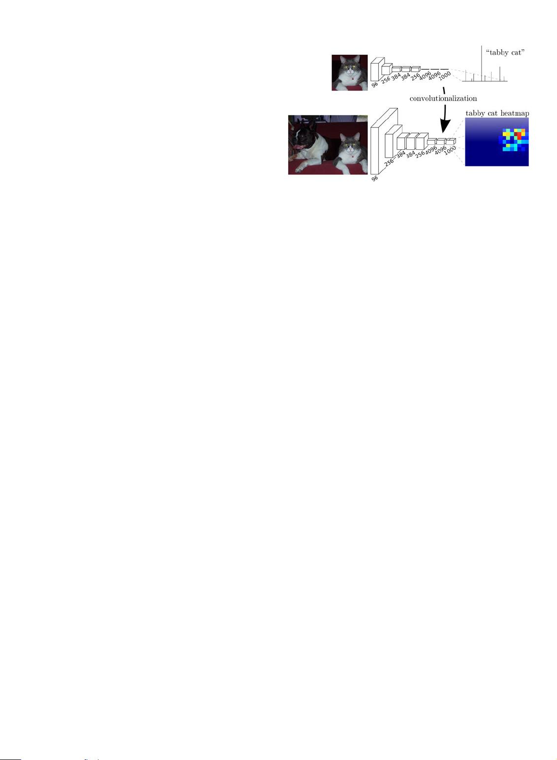
3.1 Adapting Classifiers for Dense Prediction
Typical recognition nets, including LeNet [21], AlexNet [1],
and its deeper successors [2], [3], ostensibly take fixed-sized
inputs and produce non-spatial outputs. The fully connected
layers of these nets have fixed dimensions and throw away
spatial coordinates. However, fully connected layers can also
be viewed as convolutions with kernels that cover their entire
input regions. Doing so casts these nets into fully convolu-
tional networks that take input of any size and make spatial
output maps. This transformation is illustrated in Fig. 2.
Furthermore, while the resulting maps are equivalent to
the evaluation of the original net on particular input
patches, the computation is highly amortized over the
overlapping regions of those patches. For example, while
AlexNet takes 1:2 ms (on a typical GPU) to infer the classifi-
cation scores of a 227 227 image, the fully convolutional
net takes 22 ms to produce a 10 10 grid of outputs from a
500 500 image, which is more than 5 times faster than the
na
€
ıve approach.
1
The spatial output maps of these convolutionalized mod-
els make them a natural choice for dense problems like
semantic segmentation. With ground truth available at
every output cell, both the forward and backward passes
are straightforward, and both take advantage of the inher-
ent computational efficiency (and aggressive optimization)
of convolution. The corresponding backward times for the
AlexNet example are 2:4 ms for a single image and 37 ms
for a fully convolutional 10 10 output map, resulting in a
speedup similar to that of the forward pass.
While our reinterpretation of classification nets as fully
convolutional yields output maps for inputs of any size, the
output dimensions are typically reduced by subsampling.
The classification nets subsample to keep filters small and
computational requirements reasonable. This coarsens the
output of a fully convolutional version of these nets, reduc-
ing it from the size of the input by a factor equal to the pixel
stride of the receptive fields of the output units.
Fig. 2. Transforming fully connected layers into convolution layers ena-
bles a classification net to output a spatial map. Adding differentiable
interpolation layers and a spatial loss (as in Fig. 1) produces an efficient
machine for end-to-end pixelwise learning.
1. Assuming efficient batching of single image inputs. The classifica-
tion scores for a single image by itself take 5.4 ms to produce, which is
nearly 25 times slower than the fully convolutional version.
642 IEEE TRANSACTIONS ON PATTERN ANALYSIS AND MACHINE INTELLIGENCE, VOL. 39, NO. 4, APRIL 2017


