SURF特征检测与描述技术详解

需积分: 10 139 浏览量更新于2024-07-16 收藏 1.82MB PDF 举报

"这篇资源是关于Speeded-Up Robust Features (SURF)的论文，详细介绍了这一特征检测与描述方法。SURF是一种快速、鲁棒且尺度和旋转不变的特征检测和描述算子，旨在在保持高重复性、独特性和稳健性的同时，提高计算速度。论文作者包括Herbert Baya、Andreas Essa等人，发表于2007年。" 在计算机视觉领域，特征检测和描述是图像处理和模式识别的核心部分。SURF（Speeded-Up Robust Features）作为一种高效算法，针对传统的特征提取方法进行了优化，特别是在速度和性能上有了显著提升。该算法主要由以下几个关键步骤组成： 1. **尺度空间极值检测**：SURF使用基于Hessian矩阵的检测器来寻找图像中的兴趣点。Hessian矩阵能捕捉图像的二阶导数信息，帮助确定图像局部的曲率，从而找到潜在的特征点。这种方法使得特征检测对尺度变化具有不变性。 2. **加速计算**：通过使用积分图像（Integral Image），SURF能够快速执行图像卷积操作，大大提高了计算效率。积分图像是一种预处理技术，可以有效地计算图像任意矩形区域的像素和，为特征检测提供快速路径。 3. **特征描述**：SURF采用了一种基于直方图的描述符，称为加速稳定特征向量（ASIFT）。这个描述符对特征点周围的图像块进行采样，并根据梯度方向和强度构建方向直方图，形成一个具有旋转不变性的描述子。这种方法确保了特征描述的鲁棒性，即使在光照变化和轻微几何变形下也能有效匹配。 4. **匹配步骤**：SURF通过汉明距离或其他相似度度量方法比较特征描述符，找到最佳匹配。这种匹配过程同样被优化以提高速度，确保在大规模特征数据库中快速查找。 5. **实验与评估**：论文详细探讨了各种参数对检测和描述效果的影响，以及与其他已知方法如SIFT（Scale-Invariant Feature Transform）的对比。实验结果证明，尽管速度更快，但SURF在重复性、独特性和稳健性方面并不逊色于SIFT。 SURF是计算机视觉中一种重要的特征提取算法，它通过优化计算过程和设计有效的特征描述，实现了性能与速度的平衡。在图像匹配、物体识别和三维重建等应用中，SURF都显示出了优秀的性能。这篇论文对于理解并实现这一技术具有很高的参考价值。

using integral images. The calculation time therefore is

independent of the ﬁlter size. As shown in Section 5

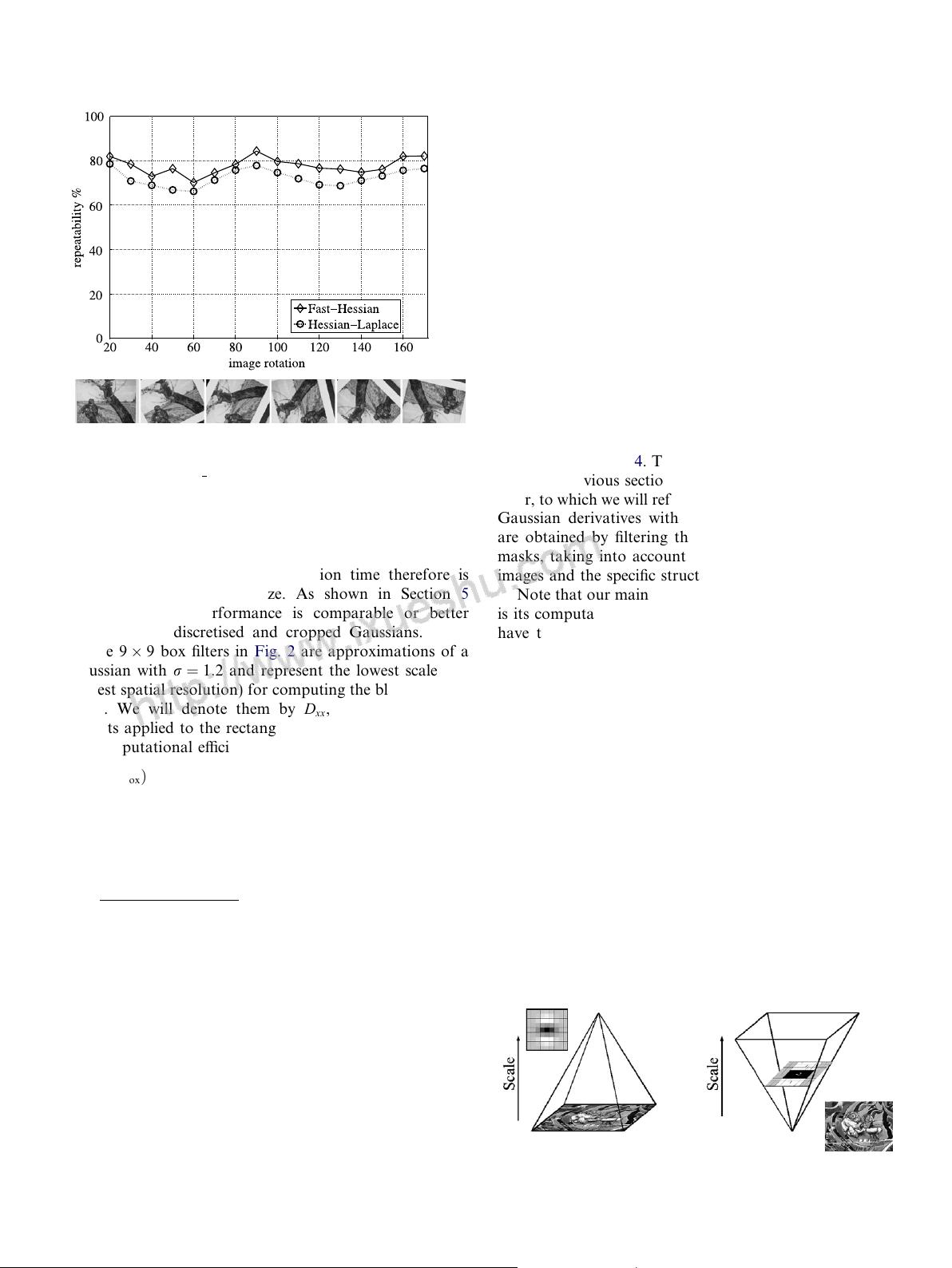
and Fig. 3, the performance is comparable or better

than with the discretised and cropped Gaussians.

The 9  9 box ﬁlters in Fig. 2 are approximations of a

Gaussian with r ¼ 1:2 and represent the lowest scale (i.e.

highest spatial resolution) for co mputing the blob response

maps. We will denote them by D

, D

, and D

. The

weights applied to the rectangular regions are kept simple

for computational eﬃciency. This yields

detðH

approx

Þ¼D

ðwD

: ð3Þ

The relative weight w of the ﬁlter responses is used to bal-

ance the expression for the Hessian’s determinant. This is

needed for the energy conservation between the Gaussian

kernels and the approximated Gaussian kernels,

w ¼

j L

ð1:2Þj

j D

ð9Þj

j L

ð1:2Þj

j D

ð9Þj

¼ 0:912::: ’ 0:9; ð4Þ

where j xj

is the Frobenius norm. Notice that for theoret-

ical correctness, the weighting changes depending on the

scale. In practice, we keep this factor constant, as this did

not have a signiﬁcant impact on the results in our

experiments.

Furthermore, the ﬁlter responses are normalised with

respect to their size. This guarantees a constant Frobenius

norm for any ﬁlter size, an important aspect for the scale

space analysis as discussed in the next section.

The approximated determinant of the Hessian repre-

sents the blob response in the image at location x. These

responses are stored in a blob response map over diﬀerent

scales, and local maxima are detected as explained in Sec-

tion 3.4.

3.3. Scale space representation

Interest points need to be found at diﬀerent scales, not

least be cause the search of correspondences often requires

their comparison in images where they are seen at diﬀerent

scales. Scale spaces are usually implemented as an image

pyramid. The images are repeatedly smoothed with a

Gaussian and then sub-sampled in order to achieve a

higher level of the pyramid. Lowe [24] subtracts these pyr-

amid layers in order to get the DoG (Diﬀerence of Gaussi-

ans) images where edges and blobs can be found.

Due to the use of box ﬁlters and integral images, we do

not have to iteratively apply the same ﬁlter to the output of

a previously ﬁltered layer, but instead can apply box ﬁlters

of any size at exactly the same speed directly on the original

image and even in parallel (although the latter is not

exploited here). Therefore, the scale space is analysed by

up-scaling the ﬁlter size rather than iteratively reducing

the image size, Fig. 4. The output of the 9  9 ﬁlter, intro-

duced in previous section, is considered as the initial scale

layer, to which we will refer as scale s ¼ 1:2 (approximating

Gaussian derivatives with r ¼ 1:2). The following layers

are obtained by ﬁltering the image with gradually bigger

masks, taking into account the discrete nature of integral

images and the speciﬁc structure of our ﬁlters.

Note that our main motivation for this type of sampling

is its computational eﬃciency. Furthermore, as we do not

have to downsample the image, there is no aliasing. On

the downside, box ﬁlters preserve high-frequency compo-

nents that can get lost in zoomed-out variants of the same

scene, which can limit scale-invariance. This was however

not noticeable in our experiments.

The scale space is divided into octaves. An octave repre-

sents a series of ﬁlter response maps obtained by convolv-

ing the same input image with a ﬁlter of increasing size. In

total, an octave encompasses a scaling factor of 2 (which

implies that one needs to more than double the ﬁlter size,

see below). Each octave is subdivided into a constant num-

ber of scale levels. Due to the discrete nature of integral

images, the minimum scale diﬀerence between two subse-

quent scales depends on the length l

of the positive or neg-

ative lobes of the partial second order derivative in the

direction of derivation (x or y), which is set to a third of

the ﬁlter size length. For the 9  9 ﬁlter, this length l

3. For two successive levels, we must increase this size by

Fig. 3. Top: Repeatability score for image rotation of up to 180°. Hessian-

based detectors have in general a lower repeatability score for angles

around odd multiples of

. Bottom: Sample images from the sequence that

was used. Fast-Hessian is the more accurate version of our detector (FH-

15), as explained in Section 3.3.

Fig. 4. Instead of iteratively reducing the image size (left), the use of

integral images allows the up-scaling of the ﬁlter at constant cost (right).

H. Bay et al. / Computer Vision and Image Understanding 110 (2008) 346–359 349

剩余15页未读，继续阅读

AI_ON

粉丝: 10
资源: 2

SURF特征检测与描述技术详解

SURF算法（Speeded Up Robust Features）

Speeded Up Robust Feature (SURF)算法的参考文献 PPT讲解和代码

Speeded-Up_Robust_Features_SURF算法全文翻译.pdf

ORB an efficient alternative to SIFT or SURF.pdf

C#+EmguCV实现SURF算法.pdf

SURF特征原理.pdf

SURF算法介绍 (3).pdf

SURF特征原理 (2).pdf

SURF算法介绍 (2).pdf

基于SURF的图像配准方法研究.pdf

最新资源