扩散模型在图像生成中超越GAN
需积分: 1 185 浏览量
更新于2024-06-25
1
收藏 37.95MB PDF 举报
"Diffusion Models Beat GANs on Image Synthesis.pdf"
本文主要探讨了扩散模型在图像合成领域超越当前最先进的生成对抗网络(GANs)的研究成果。由Prafulla Dhariwal和Alex Nichol等人发表,他们来自OpenAI,展示了如何通过一系列的消融研究找到更优的架构,提升无条件图像合成的质量。扩散模型是一种新兴的生成模型,通过逐步扩散和恢复过程来创建高逼真度的图像。
在无条件图像合成任务中,作者们通过对模型进行改进,实现了比当前最佳方法更高的图像质量。对于有条件图像合成,他们引入了分类器指导(classifier guidance)技术,这是一种高效的方法,通过利用分类器的梯度在多样性与保真度之间做出平衡。这种技术能够提高样本的质量,同时保持对分布的更好覆盖。
实验结果显示,他们的模型在ImageNet的128x128、256x256和512x512分辨率上分别达到了2.97、4.59和7.72的Fréchet Inception Distance (FID)分数,FID是一种评估生成图像质量和真实图像之间相似度的指标,数值越低表示质量越高。值得注意的是,即使每个样本仅进行25次前向传递,该模型也能与BigGAN-deep相媲美,这在计算效率上具有显著优势。
此外,作者发现分类器指导与上采样扩散模型相结合能产生更优的效果,将FID进一步降低到256x256分辨率下的3.94和512x512分辨率下的3.85。这些结果表明,扩散模型在图像合成领域的表现已经超过了传统的GANs,并且在保持高质量的同时,还能实现更高的效率和多样性。
论文最后提到,研究代码已开源,可在https://github.com/openai/guided-diffusion获取,这为其他研究者和开发者提供了深入研究和应用扩散模型的平台。
总结起来,这篇研究揭示了扩散模型在图像生成上的优越性,特别是在与分类器结合使用时,不仅提高了生成图像的逼真度,还降低了计算成本,这将推动AI和深度学习领域在图像生成技术方面的进步。同时,这也为未来研究提供了一个新的方向,即如何更好地优化和利用扩散模型,以实现更加多样化且高质量的图像合成。
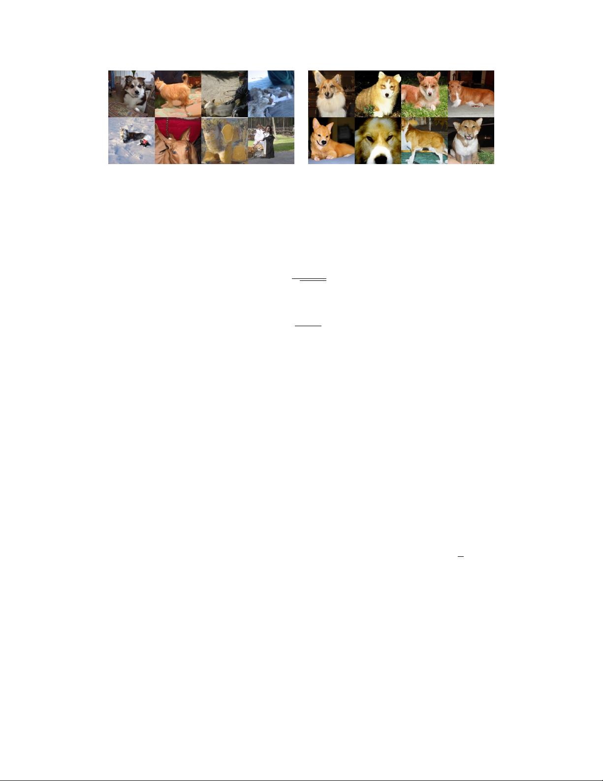
Figure 3: Samples from an unconditional diffusion model with classifier guidance to condition
on the class "Pembroke Welsh corgi". Using classifier scale 1.0 (left; FID: 33.0) does not produce
convincing samples in this class, whereas classifier scale 10.0 (right; FID: 12.0) produces much more
class-consistent images.
We can now substitute this into the score function for p(x
t
)p(y|x
t
):
∇
x
t
log(p
θ
(x
t
)p
φ
(y|x
t
)) = ∇
x
t
log p
θ
(x
t
) + ∇
x
t
log p
φ
(y|x
t
) (12)
= −
1
√
1 − ¯α
t
θ
(x
t
) + ∇
x
t
log p
φ
(y|x
t
) (13)
Finally, we can define a new epsilon prediction
ˆ(x
t
)
which corresponds to the score of the joint
distribution:
ˆ(x
t
)
:
=
θ
(x
t
) −
√
1 − ¯α
t
∇
x
t
log p
φ
(y|x
t
) (14)
We can then use the exact same sampling procedure as used for regular DDIM, but with the modified
noise predictions
ˆ
θ
(x
t
)
instead of
θ
(x
t
)
. Algorithm 2 summaries the corresponding sampling
algorithm.
4.3 Scaling Classifier Gradients
To apply classifier guidance to a large scale generative task, we train classification models on
ImageNet. Our classifier architecture is simply the downsampling trunk of the UNet model with
an attention pool [
49
] at the 8x8 layer to produce the final output. We train these classifiers on the
same noising distribution as the corresponding diffusion model, and also add random crops to reduce
overfitting. After training, we incorporate the classifier into the sampling process of the diffusion
model using Equation 10, as outlined by Algorithm 1.
In initial experiments with unconditional ImageNet models, we found it necessary to scale the
classifier gradients by a constant factor larger than 1. When using a scale of 1, we observed that the
classifier assigned reasonable probabilities (around 50%) to the desired classes for the final samples,
but these samples did not match the intended classes upon visual inspection. Scaling up the classifier
gradients remedied this problem, and the class probabilities from the classifier increased to nearly
100%. Figure 3 shows an example of this effect.
To understand the effect of scaling classifier gradients, note that
s ·∇
x
log p(y|x) = ∇
x
log
1
Z
p(y|x)
s
,
where
Z
is an arbitrary constant. As a result, the conditioning process is still theoretically grounded
in a re-normalized classifier distribution proportional to
p(y|x)
s
. When
s > 1
, this distribution
becomes sharper than
p(y|x)
, since larger values are amplified by the exponent. In other words, using
a larger gradient scale focuses more on the modes of the classifier, which is potentially desirable for
producing higher fidelity (but less diverse) samples.
In the above derivations, we assumed that the underlying diffusion model was unconditional, modeling
p(x)
. It is also possible to train conditional diffusion models,
p(x|y)
, and use classifier guidance in
the exact same way. Table 4 shows that the sample quality of both unconditional and conditional
models can be greatly improved by classifier guidance. We see that, with a high enough scale, the
guided unconditional model can get quite close to the FID of an unguided conditional model, although
training directly with the class labels still helps. Guiding a conditional model further improves FID.
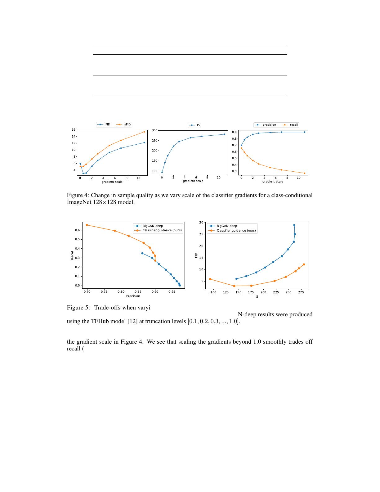
Table 4 also shows that classifier guidance improves precision at the cost of recall, thus introducing
a trade-off in sample fidelity versus diversity. We explicitly evaluate how this trade-off varies with
8
剩余43页未读,继续阅读
2024-04-03 上传
2024-07-11 上传
2019-05-08 上传
2024-07-11 上传
2019-09-07 上传
2023-04-28 上传
2024-07-11 上传
2024-07-11 上传
2023-05-18 上传

IT徐师兄
- 粉丝: 2401
- 资源: 2862
 我的内容管理
展开
我的内容管理
展开


最新资源
- 人工智能导论-拼音输入法.zip
- 协同测距matlab程序和数据.rar
- CPP.rar_人物传记/成功经验_Visual_C++_
- sslpod
- matlab拟合差值代码-PSCFit:Matlab代码,包括GUI,用于分析相和强直突触后电流(PSC)
- postman-twitter-ads-api:Twitter Ads API的Postman集合
- Cactu-Love_my-first-project
- 中英文手机网站源代码
- PscdPack:SEGA Genesis Classics ROM包装机
- 人工智能大作业-无人机图像目标检测.zip
- Advanced Image Upload and Manager Script-开源
- 00.rar_棋牌游戏_Visual_C++_
- INJECT digital creativity for journalists-crx插件
- bert_models
- HTP_SeleniumSmokeTest
- Remote Torrent Adder-crx插件
