《算法设计》Kleinberg & Tardos 教材英文版

4星 · 超过85%的资源 | 下载需积分: 50 | PDF格式 | 42.78MB | 更新于2024-08-01 | 28 浏览量 | 举报

1 收藏

"Algorithm.Design,由Kleinberg和Tardos编写的算法设计教材，是国外知名的教学材料，主要探讨算法的设计和分析。该书由Addison-Wesley在2005年出版，包含了丰富的算法理论和实践内容，旨在帮助读者理解和构建高效的计算解决方案。" 本书《Algorithm Design》是算法设计领域的经典之作，由康奈尔大学的两位著名学者Jon Kleinberg和Eva Tardos合作撰写。全书涵盖了广泛的算法主题，包括图论、动态规划、网络流、近似算法以及随机化方法等核心概念。这些算法设计技术对于解决计算机科学中的复杂问题至关重要。在图论部分，书中深入讲解了图的基本概念，如最短路径算法（Dijkstra's algorithm）和最小生成树（Prim's和Kruskal's algorithms），这些都是理解和解决网络中距离计算问题的基础。同时，书中还涵盖了网络流问题，如Ford-Fulkerson算法，这些方法在优化物流、通信网络等问题中有着广泛的应用。动态规划是算法设计中的另一个关键工具，它能够解决具有重叠子问题和最优子结构的问题。书中通过经典的背包问题、最长公共子序列等例子，让读者掌握动态规划的思想和应用。近似算法部分则讨论了如何在无法找到精确解的情况下，寻找问题的接近最优解。这在处理NP-hard问题时尤为重要，例如旅行商问题和最大独立集问题。书中详细介绍了多项式时间内的近似算法设计技巧。随机化算法是近年来发展迅速的领域，Kleinberg和Tardos在书中阐述了这一方法如何在概率上下文中提供高效解决方案，如快速排序（QuickSort）和鸽巢原理（Pigeonhole Principle）的应用。此外，书中还包括了大量实例、习题和案例研究，以帮助读者将理论知识转化为实际问题的解决方案。这些练习涵盖了各种难度，从基础到高级，适合不同层次的学习者。《Algorithm Design》是学习和提升算法设计能力的宝贵资源，无论对于计算机科学的学生还是专业的软件工程师，都能从中受益匪浅。通过阅读此书，读者可以系统地学习和掌握算法设计的精髓，从而在面对复杂的计算挑战时能够游刃有余。

Chapter 1 Introduction: Some Representative Problems

1.1 A First Problem: Stable Matching

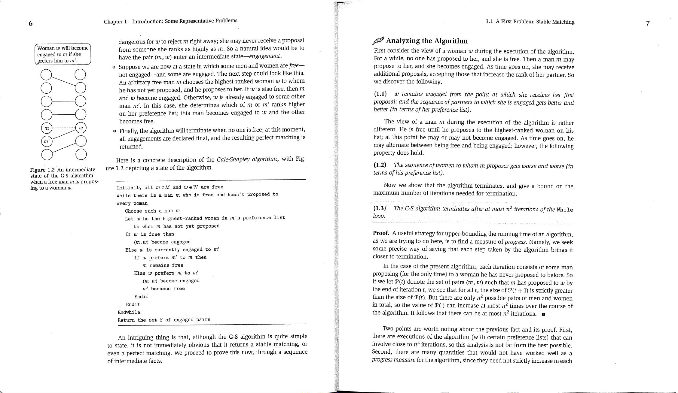
oman w will become~

ngaged to m if she

refers him to rat

Figure 1.2 An intermediate

state of the G-S algorithm

when a free man ra is propos-

ing to a woman w.

dangerous for w to reject m right away; she may never receive a proposal

from someone she ranks as highly as m. So a natural idea would be to

have the pair

(m, w)

enter an intermediate

state--engagement.

Suppose we are now at a state in which some men and women are/Tee--

not engaged--and some are engaged. The next step could look like this.

An arbitrary flee man m chooses the highest-ranked woman w to whom

he has not yet proposed, and he proposes to her. If w is also free, then m

and w become engaged. Otherwise, w is already engaged to some other

man m’. In this case, she determines which of m or m’ ranks higher

on her preference list; this man becomes engaged to w and the other

becomes flee,

Finally, the algorithm wil! terminate when no one is free; at this moment,

all engagements are declared final, and the resulting perfect matchdng is

returned.

Here is a concrete description of the

Gale-Shapley algorithm, with

Fig-

ure 1.2 depicting a state of the algorithm.

Initially all m E M and w E W are free

While there is a man m who is free and hasn’t proposed to

every woman

Choose such a man m

Let w be the highest-ranked woman in m’s preference list

to whom m has not yet proposed

If ~ is free then

(m, ~) become engaged

Else ~ is currently engaged to m’

If ~ prefers m’ to m then

m remains free

Else w prefers m to m’

(m,~) become engaged

becomes free

Endif

Endwhile

Return the set S of engaged pairs

An intriguing thing is that, although the G-S algorithm is quite simple

to state, it is not immediately obvious that it returns a stable matching, or

even a perfect matching. We proceed to prove this now, through a sequence

of intermediate facts.

~ Analyzing the Algorithm

First consider the view of a woman w during the execution of the algorithm.

For a while, no one has proposed to her, and she is free. Then a man m may

propose to her, and she becomes engaged. As time goes on, she may receive

additional proposals, accepting those that increase the rank of her partner. So

we discover the following.

(1.1)

w remains engaged /Tom the point at which she receives her first

proposal; and the sequence of partners to which she is engaged gets better and

better (in terms of her preference list).

The view of a man m during the execution of the algorithm is rather

different. He is free until he proposes to the highest-ranked woman on his

list; at this point he may or may not become engaged. As time goes on, he

may alternate between being free and being engaged; however, the following

property does hold.

(1.2)

The sequence of women to whom m proposes gets worse and worse (in

terms of his preference list).

Now we show that the algorithm terminates, and give a bound on the

maximum number of iterations needed for termination.

(1,3)

The G-S algorithm terminates after at most n

iterations of the

While

loop.

Proof. A useful strategy for upper-bounding the running time of an algorithm,

as we are trying to do here, is to find a measure of

progress.

Namely, we seek

some precise way of saying that each step taken by the algorithm brings it

closer to termination.

In the case of the present algorithm, each iteration consists of some man

proposing (for the only time) to a woman he has never proposed to before. So

if we let ~P(t) denote the set of pairs

(m, w)

such that m has proposed to w by

the end of iteration

we see that for all

t, the

size of ~P(t + 1) is strictly greater

than the size of ~P(t). But there are only n

possible pairs of men and women

in total, so the value of ~P(.) can increase at most n

times over the course of

the algorithm. It follows that there can be at most n

iterations. []

Two points are worth noting about the previous fact and its proof. First,

there are executions of the algorithm (with certain preference lists) that can

involve close to n

iterations, so this analysis is not far from the best possible.

Second, there are many quantities that would not have worked well as a

progress measure

for the algorithm, since they need not strictly increase in each

Chapter 1 Introduction: Some Representative Problems

1.1 A First Problem: Stable Matching

iteration. For example, the number of free individuals could remain constant

from one iteration to the next, as could the number of engaged pairs. Thus,

these quantities could not be used directly in giving an upper bound on the

maximum possible number of.iterations, in the style of the previous paragraph.

Let us now establish that the set S returned at the termination of the

algorithm is in fact a perfect matching. Why is this not immediately obvious?

Essentially, we have to show that no man can

"fall

off" the end of his preference

list; the only way for the ~’h±].e loop to exit is for there to be no flee man. In

this case, the set of engaged couples would indeed be a perfect matching.

So the main thing we need to show is the following.

(1.4)

If m is free at some point in the execution of the algorithm, then there

is a woman to whom he has not yet proposed.

Proof. Suppose there comes a point when m is flee but has already proposed

to every woman. Then by (1.1), each of the n women is engaged at this point

in time. Since the set of engaged pairs forms a matching, there must also be

n engaged men at this point in time. But there are only n men total, and m is

not engaged, so this is a contradiction.

(1..~)

The set S returned at termination is a peryect matching.

Proof. The set of engaged pairs always forms a matching. Let us suppose that

the algorithm terminates with a flee man m. At termination, it must be the

case that m had already proposed to every woman, for otherwise the ~qhile

loop would not have exited. But this contradicts (1.4), which says that there

cannot be a flee man who has proposed to every woman.

Finally, we prove the main property of the algorithm--namely, that it

results in a stable matching.

(1.6)

Consider an executionof the G-S algorithm that returns a set of pairs

S. The set S is a stable matching.

Proof. We have already seen, in (1.5), that S is a perfect matching. Thus, to

prove S is a stable matching, we will assume that there is an instability with

respect to S and obtain a contradiction. As defined earlier, such an instability

would involve two pairs,

(m, w)

and (m’, w’), in S with the properties that

o m prefers w’ to w, and

o w’ prefers m to mL

In the execution of the algorithm that produced S, m’s last proposal was, by

definition, to w. Now we ask: Did m propose to w’ at some earlier point in

this execution? If he didn’t, then w must occur higher on

m’s

preference.list

than w’,

contxadicting our assumption that m prefers w’ to w. If he did, then

he was rejected by w’ in favor of some other man

m",

whom w’ prefers to m.

m’

is the final partner of

w’,

so either m" = m’ or, by (1.!), w’ prefers her final

partner m

to m"; either way this contradicts our assumption that w’ prefers

m to m

It follows that S is a stable matching. []

Extensions

We began by defining the notion of a stable matching; we have just proven

that the G-S algorithm actually constructs one. We now consider some further

questions about the behavior of the G-S algorithm and its relation to the

properties of different stable matchings.

To begin wit_h, recall that we saw an example earlier in which there could

be multiple stable matchings. To recap, the preference lists in this example

were as follows:

prefers w to w’.

prefers w’ to w.

prefers m

to m.

prefers m to m’.

Now, in any execution of the Gale-Shapley algorithm, m will become engaged

w, m’ will become engaged to w’ (perhaps in the other order), and things

will stop there. Thus, the

other

stable matching, consisting of the pairs

(m’, w)

and

(m, w’),

is not attainable from an execution of the G-S algorithm in which

the men propose. On the other hand, it would be reached if we ran a version of

the algorithm in which the women propose. And in larger examples, with more

than two people on each side, we can have an even larger collection of possible

stable matchings, many of them not achievable by any natural algorithm.

This example shows a certain "unfairness" in the G-S algorithm, favoring

men. If the men’s preferences mesh perfectly (they all list different women as

their first choice), then in all runs of the G-S algorithm all men end up matched

with their first choice, independent of the preferences of the women. If the

women’s preferences clash completely with the men’s preferences (as was the

case in this example), then the resulting stable matching is as bad as possible

for the women. So this simple set of preference lists compactly summarizes a

world in which

someone

is destined to end up unhappy: women are unhappy

if men propose, and men are unhappy if women propose.

Let’s now analyze the G-S algorithm in more detail and try to understand

how general this "unfairness" phenomenon is.

Chapter 1 Introduction: Some Representative Problems

To begin With, our example reinforces the point that the G-S algorithm

is actually underspecified: as long as there is a free man, we are allowed to

choose any flee man to make the next proposal. Different choices specify

different executions of the algprithm; this is why, to be careful, we stated (1.6)

as "Consider an execution of the G-S algorithm that returns a set of pairs

S,"

instead of "Consider the set S returned by the G-S algorithm."

Thus, we encounter another very natural question: Do all executions of

the G-S algorithm yield the same matching? This is a genre of question that

arises in many settings in computer science: we have an algorithm that runs

asynchronously,

with different independent components performing actions

that can be interleaved in complex ways, and we want to know how much

variability this asynchrony causes in the final outcome. To consider a very

different kind of example, the independent components may not be men and

women but electronic components activating parts of an airplane wing; the

effect of asynchrony in their behavior can be a big deal.

In the present context, we will see that the answer to our question is

surprisingly clean: all executions of the G-S algorithm yield the same matching.

We proceed to prove this now.

All Executions Yield the Same Matching

There are a number of possible

ways to prove a statement such as this, many of which would result in quite

complicated arguments. It turns out that the easiest and most informative ap-

proach for us will be to uniquely

characterize the

matching that is obtained and

then show that al! executions result in the matching with this characterization.

What is the characterization? We’ll show that each man ends up with the

"best possible partner" in a concrete sense. (Recall that this is true if all men

prefer different women.) First, we will say that a woman iv is a

valid partner

of a man m if there is a stable matching that contains the pair

(m, iv).

We will

say that iv is the

best valid partner

of m if iv is a valid parmer of m, and no

woman whom m ranks higher than iv is a valid partner of his. We will use

best(m)

to denote the best valid partner of m.

Now, let S* denote the set of pairs {(m,

best(m)) : m ~ M}.

We will prove

the folloWing fact.

(1.7)

Every execution of the C--S algorithm results in the set S*:

This statement is surprising at a number of levels. First of all, as defined,

there is no reason to believe that S* is a matching at all, let alone a stable

matching. After all, why couldn’t it happen that two men have the same best

valid partner? Second, the result shows that the G-S algorithm gives the best

possible outcome for every man simultaneously; there is no stable matching

in which any of the men could have hoped to do better. And finally, it answers

1.1 A First Problem: Stable Matching

our question above by showing that the order of proposals in the G-S algorithm

has absolutely no effect on the final outcome.

Despite all this, the proof is not so difficult.

Proof. Let us suppose, by way of contradiction, that some execution g of the

G-S algorithm results in a matching S in which some man is paired with a

woman who is not his best valid partner. Since men propose in decreasing

order of preference, this means that some man is rejected by a valid partner

during the execution g of the algorithm. So consider the first moment during

the execution g in which some man, say m, is rejected by a valid partner iv.

Again, since men propose in decreasing order of preference, and since this is

the first time such a rejection has occurred, it must be that iv is m’s best valid

partner

best(m).

The reiection of m by iv may have happened either because m proposed

and was turned down in favor of iv’s existing engagement, or because iv broke

her engagement to m in favor of a better proposal. But either way, at this

moment iv forms or continues an engagement with a man m’ whom she prefers

to m.

Since iv is a valid parmer of m, there exists a stable matching S’ containing

the pair (m, iv).

Now we ask: Who is m’ paired with in this matching? Suppose

it is a woman

iv’ ~= iv.

Since the rejection of m by iv was the first rejection of a man by a valid

partner in the execution ~, it must be that m’ had not been rejected by any valid

parmer at the point in ~ when he became engaged to iv. Since he proposed in

decreasing order of preference, and since iv’ is clearly a valid parmer of m’,

must be that m’ prefers iv to

iv’.

But we have already seen that iv prefers m’

to m, for in execution ~ she rejected m in favor of m’. Since (m’, iv) 

S’,

follows that (m’, iv) is an instability in S’.

This contradicts our claim that S’ is stable and hence contradicts our initial

assumption. []

So for the men, the G-S algorithm is ideal. Unfortunately, the same cannot

be said for the women. For a woman w, we say that m is a valid partner if

there is a stable matching that contains the pair (m, w). We say that m is the

ivorst valid partner

of iv if m is a valid partner of

and no man whom iv

ranks lower than m is a valid partner of hers.

(1.8)

In the stable matching S*, each woman is paired ivith her ivorst valid

partner.

Proof.

Suppose there were a pair (m, iv) in S* such that m is not the worst

valid partner of iv. Then there is a stable matching S’ in which iv is paired

Chapter

1 Introduction: Some Representative Problems

with a man m’ whom she likes less than m. In S’, m is paired with a woman

w’ ~ w; since w is the best valid partner of m, and w’ is a valid partner of

we see that m prefers w to w’.

But from this it follows that (m, w) is an instability in S’, contradicting the

claim that S’ is stable and hence contradicting our initial assumption. []

Thus, we find that our simple example above, in which the men’s pref-

erences clashed with the women’s, hinted at a very general phenomenon: for

any input, the side that does the proposing in the G-S algorithm ends up with

the best possible stable matching (from their perspective), while the side that

does not do the proposing correspondingly ends up with the worst possible

stable matching.

1.2 Five Representative Problems

The Stable Matching Problem provides us with a rich example of the process of

algorithm design. For many problems, this process involves a few significant,

steps: formulating the problem with enough mathematical precision that we

can ask a concrete question and start thinking about algorithms to solve

it; designing an algorithm for the problem; and analyzing the algorithm by

proving it is correct and giving a bound on the running time so as to establish

the algorithm’s efficiency.

This high-level strategy is carried out in practice with the help of a few

fundamental design techniques, which are very useful in assessing the inherent

complexity of a problem and in formulating an algorithm to solve it. As in any

area, becoming familiar with these design techniques is a gradual process; but

with experience one can start recognizing problems as belonging to identifiable

genres and appreciating how subtle changes in the statement of a problem can

have an enormous effect on its computational difficulty.

To get this discussion started, then,, it helps to pick out a few representa-

tive milestones that we’ll be encountering in our study of algorithms: cleanly

formulated problems, all resembling one another at a general level, but differ-

ing greatly in their difficulty and in the kinds of approaches that one brings

to bear on them. The first three will be solvable efficiently by a sequence of

increasingly subtle algorithmic techniques; the fourth marks a major turning

point in our discussion, serving as an example of a problem believed to be un-

solvable by any efficient algorithm; and the fifth hints at a class of problems

believed to be harder stil!.

The problems are self-contained and are al! motivated by computing

applications. To talk about some of them, though, it will help to use the

termino!ogy of

graphs.

While graphs are a common topic in earlier computer

1.2 Five Representative Problems

science courses, we’ll be introducing them in a fair amount of depth in

Chapter 3; due to their enormous expressive power, we’ll also be using them

extensively throughout the book. For the discussion here, it’s enough to think

of a graph G as simply a way of encoding pairwise relationships among a set

of objects. Thus, G consists of a pair of sets

(V,

E)--a collection V of

nodes

and a collection E of

edges, each of which "joins" two of the nodes. We thus

represent an edge e ~ E as a two-element subset of V: e =

(u, u)

for some

u, u ~ V,

where we call u and u the

ends

of e. We typica!ly draw graphs as in

Figure 1.3, with each node as a small circle and each edge as a line segment

joining its two ends.

Let’s now turn to a discussion of the five representative problems.

Interval Scheduling

Consider the following very simple scheduling problem. You have a resource--

it may be a lecture room, a supercompnter, or an electron microscope--and

many people request to use the resource for periods of time. A

request

takes

the form: Can I reserve the resource starting at time

until time f? We will

assume that the resource can be used by at most one person at a time. A

scheduler wants to accept a subset of these requests, rejecting al! others, so

that the accepted requests do not overlap in time. The goal is to maximize the

number of requests accepted.

More formally, there will be n requests labeled 1 ..... n, with each request

i specifying a start time

and a finish time fi. Naturally, we have si < fi for all

i. Two requests i andj are

compatible

if the requested intervals do not overlap:

that is, either request i is for an earlier time interval than request

j (fi

or request i is for a later time than request j (1~ _< si). We’ll say more generally

that a subset A of requests is compatible if all pairs of requests

i,j ~ A, i ~=j are

compatible. The goal is to select a compatible subset of requests of maximum

possible size.

We illustrate an instance of this

Interual Scheduling Problem

in Figure 1.4.

Note that there is a single compatible set of size 4, and this is the largest

compatible set.

Figure 1.4 An instance of the Interval Scheduling Problem.

(a)

Figure 1.3 Each of (a) and

(b) depicts a graph on four

nodes.

Chapter ! Introduction: Some Representative Problems

We will see shortly that this problem can be solved by a very natural

algorithm that orders the set of requests according to a certain heuristic and

then "greedily" processes them in one pass, selecting as large a compatible

subset as it can. This will be .typical of a class of

greedy algorithms

that we

will consider for various problems--myopic rules that process the input one

piece at a time with no apparent look-ahead. When a greedy algorithm can be

shown to find an optimal solution for al! instances of a problem, it’s often fairly

surprising. We typically learn something about the structure of the underlying

problem from the fact that such a simple approach can be optimal.

Weighted Interval Scheduling

In the Interval Scheduling Problem, we sohght to maximize the

number

requests that could be accommodated simultaneously. Now, suppose more

generally that each request interval i has an associated

value,

weight,

vi > O; we could picture this as the amount of money we will make from

the

individual if we schedule his or her request. Our goal will be to find a

compatible subset of intervals of maximum total value.

The case in which vi = I for each i is simply the basic Interval Scheduling

Problem; but the appearance of arbitrary values changes the nature of the

maximization problem quite a bit. Consider, for example, that if v

exceeds

the sum of all other vi, then the optimal solution must include interval 1

regardless of the configuration of the fi~l set of intervals. So any algorithm

for this problem must be very sensitive to the values, and yet degenerate to a

method for solving (unweighted) interval scheduling when all the values are

equal to 1.

There appears to be no simple greedy rule that walks through the intervals

one at a time, making the correct decision in the presence of arbitrary values.

Instead, we employ a technique,

dynamic programming,

that builds up the

optimal value over all possible solutions in a compact, tabular way that leads

to a very efficient algorithm.

Bipal~te Matching

When we considered the Stable Matching Problem, we defined a

matching

be a set of ordered pairs of men and women with the property that each man

and each woman belong to at most one of the ordered pairs. We then defined

a perfect matching to be a matching in which every man and every woman

belong to some pair.

We can express these concepts more generally in terms of graphs, and in

order to do this it is useful to define the notion of a

bipartite graph.

We say that

a graph G ---- (V, E) is

bipa~te

if its node set V can be partitioned into sets X

1.2 Five Representative Problems

and Y in such a way that every edge has one end in X and the other end in Y.

A bipartite graph is pictured in Figure 1.5; often, when we want to emphasize

a graph’s "bipartiteness," we will draw it this way, with the nodes in X and

Y in two parallel columns. But notice, for example, that the two graphs in

Figure 1.3 are also bipartite.

Now, in the problem of finding a stable matching, matchings were built

from pairs of men and women. In the case of bipartite graphs, the edges are

pairs of nodes, so we say that a matching in a graph G = (V, E) is a set of edges

M _c E with the property that each node appears in at most one edge of M.

M is a perfect matching if every node appears in exactly one edge of M.

To see that this does capture the same notion we encountered in the Stable

Matching Problem, consider a bipartite graph G’ with a set X of n men, a set Y

of n women, and an edge from every node in X to every node in Y. Then the

matchings and perfect matchings in G’ are precisely the matchings and perfect

matchings among the set of men and women.

In the Stable Matching Problem, we added preferences to this picture. Here,

we do not consider preferences; but the nature of the problem in arbitrary

bipartite graphs adds a different source of complexity: there is not necessarily

an edge from every x ~ X to every y ~ Y, so the set of possible matchings has

quite a complicated structure. In other words, it is as though only certain pairs

of men and women are willing to be paired off, and we want to figure out

how to pair off many people in a way that is consistent with this. Consider,

for example, the bipartite graph G in Figure 1.5: there are many matchings in

G, but there is only one perfect matching. (Do you see it?)

Matchings in bipartite graphs can model situations in which objects are

being

assigned

to other objects. Thus, the nodes in X can represent jobs, the

nodes in Y can represent machines, and an edge (x~, y]) can indicate that

machine y] is capable of processing job xi. A perfect matching is then a way

of assigning each job to a machine that can process it, with the property that

each machine is assigned exactly one job. In the spring, computer science

departments across the country are often seen pondering a bipartite graph in

which X is the set of professors in the department, Y is the set of offered

courses, and an edge (xi, yj) indicates that professor x~ is capable of teaching

course y]. A perfect matching in this graph consists of an assignment of each

professor to a course that he or she can teach, in such a way that every course

is covered.

Thus the

Bipartite Matching Problem

is the following: Given an arbitrary

bipartite graph

find a matching of maximum size. If IXI = I YI = n, then there

is a perfect matching if and only if the maximum matching has size n. We will

find that the algorithmic techniques discussed earlier do not seem adequate

Figure 1.5 A bipartite graph.

剩余431页未读，继续阅读

Cheng_Tian

粉丝: 20

《算法设计》Kleinberg & Tardos 教材英文版

Algorithm Design(算法设计)中英 带目录

J. Kleinberg, E. Tardos. Algorithm Design.pdf

算法设计与分析（Algorithm Design ）课后习题作业

j. kleinberg and e. tardos. algorithm design. pearson education, 2006.

jon kleinberg and eva tardos. algorithm design答案

No module named 'pyrs.algorithm'

algorithm.algorithm_variant.tactic

连接主机... Algorithm negotiation fail

jasypt.encryptor.algorithm

最新资源

Algorithm Design(算法设计)中英带目录