模式识别经典：Richard Duda的《Pattern Classification》第二版

需积分: 9 42 浏览量更新于2024-07-24 收藏 11.28MB PDF 举报

"Richard O. Duda的《Pattern Classification》是模式识别领域的经典教材，英文原版第二版，常被用于国外大学的模式识别课程。本书涵盖了机器感知、特征提取、噪声处理、过拟合、模型选择等多个模式分类的子问题，并深入探讨了学习与适应的不同类型，如监督学习、无监督学习和强化学习。" 在模式分类领域，Richard Duda的著作深入浅出地介绍了这一主题。首先，书中提到机器感知是模式识别的基础，它涉及到如何让计算机理解和解释来自不同感官通道的信息。通过一个例子，作者引出了模式识别涉及的相关领域，包括信号处理、统计学、人工智能等。接着，Duda详细阐述了模式分类的子问题。特征提取是将原始数据转换成有意义的表示，这是预处理的关键步骤。噪声的存在可能干扰这一过程，因此需要有效的噪声处理策略。过拟合是训练模型时常见的问题，它可能导致模型在新数据上的表现不佳。模型选择则涉及到如何在多个模型中找到最佳的平衡点，以适应特定任务。此外，书中的先验知识讨论了利用先验信息来指导分类决策的重要性，而缺失特征处理则探讨了在数据不完整的情况下进行分类的方法。 Mereology（部分与整体的关系）和分割是图像分析中常见的概念，它们帮助我们理解对象的结构和边界。上下文信息对于理解模式的含义至关重要，尤其是在自然语言处理和图像识别中。不变性指的是模型应能识别出在不同变换下的同一模式，如旋转或缩放。证据聚合则涉及如何结合多个证据源来做出更准确的决策。成本和风险的考虑使我们能够权衡错误分类的后果。最后，计算复杂性分析了算法的效率，这对于实际应用中的可扩展性和资源管理至关重要。在学习与适应章节，Duda区分了三种主要的学习方式：监督学习，其中模型根据已知输入和输出对进行训练；无监督学习，模型试图从没有标签的数据中发现结构；以及强化学习，通过与环境的交互来优化决策策略。每一章的总结帮助读者回顾关键概念，而参考文献和历史评论提供了深入研究的路径。全书内容丰富，对于希望深入理解模式识别理论和技术的读者来说是一本不可或缺的参考资料。

4 CHAPTER 1. INTRODUCTION

images — variations in lighting, position of the ﬁsh on the conveyor, even “static”

due to the electronics of the camera itself.

Given that there truly are diﬀerences between the population of sea bass and that

of salmon, we view them as having diﬀerent models — diﬀerent descriptions, whichmodel

are typically mathematical in form. The overarching goal and approach in pattern

classiﬁcation is to hypothesize the class of these models, process the sensed data

to eliminate noise (not due to the models), and for any sensed pattern choose the

model that corresponds best. Any techniques that further this aim should be in the

conceptual toolbox of the designer of pattern recognition systems.

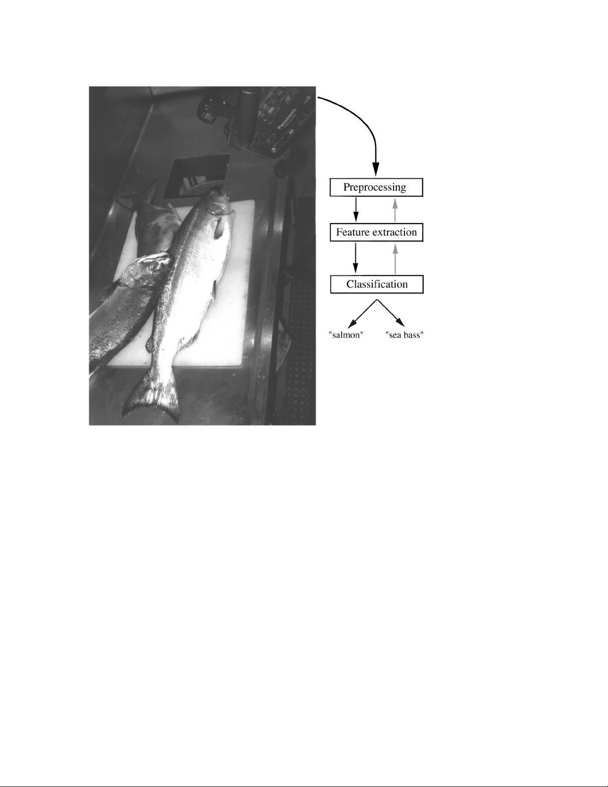
Our prototype system to perform this very speciﬁc task might well have the form

shown in Fig. 1.1. First the camera captures an image of the ﬁsh. Next, the camera’s

signals are preprocessed to simplify subsequent operations without loosing relevantpre-

processing information. In particular, we might use a segmentation operation in which the images

segmentation

of diﬀerent ﬁsh are somehow isolated from one another and from the background. The

information from a single ﬁsh is then sent to a feature extractor, whose purpose is to

feature

extraction

reduce the data by measuring certain “features” or “properties.” These features

(or, more precisely, the values of these features) are then passed to a classiﬁer that

evaluates the evidence presented and makes a ﬁnal decision as to the species.

The preprocessor might automatically adjust for average light level, or threshold

the image to remove the background of the conveyor belt, and so forth. For the

moment let us pass over how the images of the ﬁsh might be segmented and consider

how the feature extractor and classiﬁer might be designed. Suppose somebody at the

ﬁsh plant tells us that a sea bass is generally longer than a salmon. These, then,

give us our tentative models for the ﬁsh: sea bass have some typical length, and this

is greater than that for salmon. Then length becomes an obvious feature, and we

might attempt to classify the ﬁsh merely by seeing whether or not the length l of

a ﬁsh exceeds some critical value l

∗

. To choose l

∗

we could obtain some design or

training samples of the diﬀerent types of ﬁsh, (somehow) make length measurements,training

samples and inspect the results.

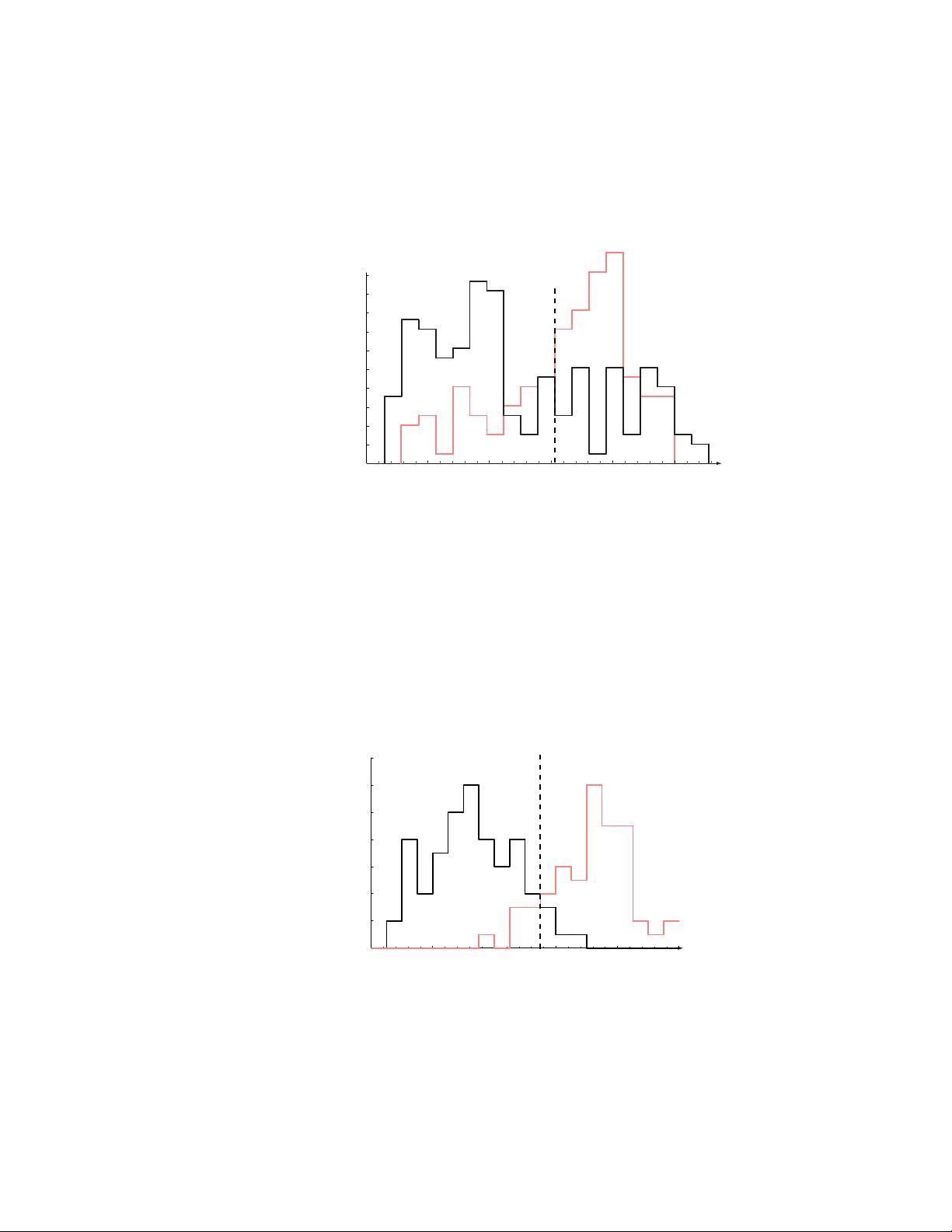
Suppose that we do this, and obtain the histograms shown in Fig. 1.2. These

disappointing histograms bear out the statement that sea bass are somewhat longer

than salmon, on average, but it is clear that this single criterion is quite poor; no

matter how we choose l

∗

, we cannot reliably separate sea bass from salmon by length

alone.

Discouraged, but undeterred by these unpromising results, we try another feature

— the average lightness of the ﬁsh scales. Now we are very careful to eliminate

variations in illumination, since they can only obscure the models and corrupt our

new classiﬁer. The resulting histograms, shown in Fig. 1.3, are much more satisfactory

— the classes are much better separated.

So far we have tacitly assumed that the consequences of our actions are equally

costly: deciding the ﬁsh was a sea bass when in fact it was a salmon was just as

undesirable as the converse. Such a symmetry in the cost is often, but not invariablycost

the case. For instance, as a ﬁsh packing company we may know that our customers

easily accept occasional pieces of tasty salmon in their cans labeled “sea bass,” but

they object vigorously if a piece of sea bass appears in their cans labeled “salmon.”

If we want to stay in business, we should adjust our decision boundary to avoid

antagonizing our customers, even if it means that more salmon makes its way into

the cans of sea bass. In this case, then, we should move our decision boundary x

∗

smaller values of lightness, thereby reducing the number of sea bass that are classiﬁed

as salmon (Fig. 1.3). The more our customers object to getting sea bass with their

1.2. AN EXAMPLE 7

2 4 6 8 10

Width

Lightness

salmon sea bass

Figure 1.4: The two features of lightness and width for sea bass and salmon. The

dark line might serve as a decision boundary of our classiﬁer. Overall classiﬁcation

error on the data shown is lower than if we use only one feature as in Fig. 1.3, but

there will still be some errors.

of more than one feature at a time.

In our search for other features, we might try to capitalize on the observation that

sea bass are typically wider than salmon. Now we have two features for classifying

ﬁsh — the lightness x

and the width x

. If we ignore how these features might be

measured in practice, we realize that the feature extractor has thus reduced the image

of each ﬁsh to a point or feature vector x in a two-dimensional feature space, where

x =





Our problem now is to partition the feature space into two regions, where for all

patterns in one region we will call the ﬁsh a sea bass, and all points in the other we

call it a salmon. Suppose that we measure the feature vectors for our samples and

obtain the scattering of points shown in Fig. 1.4. This plot suggests the following rule

for separating the ﬁsh: Classify the ﬁsh as sea bass if its feature vector falls above the

decision boundary shown, and as salmon otherwise. decision

boundary

This rule appears to do a good job of separating our samples and suggests that

perhaps incorporating yet more features would be desirable. Besides the lightness

and width of the ﬁsh, we might include some shape parameter, such as the vertex

angle of the dorsal ﬁn, or the placement of the eyes (as expressed as a proportion of

the mouth-to-tail distance), and so on. How do we know beforehand which of these

features will work best? Some features might be redundant: for instance if the eye

color of all ﬁsh correlated perfectly with width, then classiﬁcation performance need

not be improved if we also include eye color as a feature. Even if the diﬃculty or

computational cost in attaining more features is of no concern, might we ever have

too many features?

Suppose that other features are too expensive or expensive to measure, or provide

little improvement (or possibly even degrade the performance) in the approach de-

scribed above, and that we are forced to make our decision based on the two features

in Fig. 1.4. If our models were extremely complicated, our classiﬁer would have a

decision boundary more complex than the simple straight line. In that case all the

8 CHAPTER 1. INTRODUCTION

2 4 6 8 10

Width

Lightness

salmon sea bass

Figure 1.5: Overly complex models for the ﬁsh will lead to decision boundaries that are

complicated. While such a decision may lead to perfect classiﬁcation of our training

samples, it would lead to poor performance on future patterns. The novel test point

marked ? is evidently most likely a salmon, whereas the complex decision boundary

shown leads it to be misclassiﬁed as a sea bass.

training patterns would be separated perfectly, as shown in Fig. 1.5. With such a

“solution,” though, our satisfaction would be premature because the central aim of

designing a classiﬁer is to suggest actions when presented with novel patterns, i.e.,

ﬁsh not yet seen. This is the issue of generalization. It is unlikely that the complexgeneral-

ization decision boundary in Fig. 1.5 would provide good generalization, since it seems to be

“tuned” to the particular training samples, rather than some underlying characteris-

tics or true model of all the sea bass and salmon that will have to be separated.

Naturally, one approach would be to get more training samples for obtaining a

better estimate of the true underlying characteristics, for instance the probability

distributions of the categories. In most pattern recognition problems, however, the

amount of such data we can obtain easily is often quite limited. Even with a vast

amount of training data in a continuous feature space though, if we followed the

approach in Fig. 1.5 our classiﬁer would give a horrendously complicated decision

boundary — one that would be unlikely to do well on novel patterns.

Rather, then, we might seek to “simplify” the recognizer, motivated by a belief

that the underlying models will not require a decision boundary that is as complex as

that in Fig. 1.5. Indeed, we might be satisﬁed with the slightly poorer performance

on the training samples if it means that our classiﬁer will have better performance

on novel patterns.

∗

But if designing a very complex recognizer is unlikely to give

good generalization, precisely how should we quantify and favor simpler classiﬁers?

How would our system automatically determine that the simple curve in Fig. 1.6

is preferable to the manifestly simpler straight line in Fig. 1.4 or the complicated

boundary in Fig. 1.5? Assuming that we somehow manage to optimize this tradeoﬀ,

can we then predict how well our system will generalize to new patterns? These are

some of the central problems in statistical pattern recognition.

For the same incoming patterns, we might need to use a drastically diﬀerent cost

∗

The philosophical underpinnings of this approach derive from William of Occam (1284-1347?), who

advocated favoring simpler explanations over those that are needlessly complicated — Entia non

sunt multiplicanda praeter necessitatem (“Entities are not to be multiplied without necessity”).

Decisions based on overly complex models often lead to lower accuracy of the classiﬁer.

剩余737页未读，继续阅读

pengare

粉丝: 0

模式识别经典：Richard Duda的《Pattern Classification》第二版

最新资源