利用跳跃池化与RNN在场景中精确检测物体

需积分: 10 120 浏览量更新于2024-09-08 收藏 1.68MB PDF 举报

"使用跳跃池化和RNN在场景中检测物体——Inside-OutsideNet:DetectingObjectsinContextwithSkipPoolingandRecurrentNeuralNetworks" 本文深入探讨了如何利用上下文信息和多尺度表示来提高物体检测的准确性，具体通过引入Inside-OutsideNet（ION）这一对象检测框架实现。ION的独特之处在于它不仅考虑了目标区域内部的信息，还利用了外部的上下文信息。外部上下文信息的整合是通过空间循环神经网络（RNN）来完成的，这使得模型能够理解和处理场景中的复杂关系。在ION中，跳跃池化（Skip Pooling）技术被用于提取目标区域内部不同尺度和抽象层次的信息。跳跃池化允许模型在不同分辨率的特征图之间跳跃，从而捕捉到不同粒度的细节，这对于识别物体的多种形态和变体至关重要。这种技术与传统的池化操作相比，能更有效地保留空间信息，有助于物体检测任务中的定位和分类。文章通过大量实验对设计空间进行了评估，并提供了关于关键技巧的概述，揭示了哪些技术对于提高性能最为重要。实验结果表明，ION在PASCAL VOC 2012物体检测任务上的平均精度（mAP）从73.9%提升到了76.4%，在更具挑战性的MS COCO数据集上，mAP更是从19.7%提高到了33.1%，显著超越了当时的状态-of-the-art方法。在2015年的MS COCO检测挑战赛中，ION模型赢得了最佳学生参赛作品奖，并在比赛中取得了优异成绩。此外，ION的性能提升还体现在它对物体检测的全面理解上，包括物体的相对位置、大小和遮挡情况。通过RNN的递归特性，ION能够处理复杂的场景结构，识别出物体之间的相互作用，从而提高检测的准确性和鲁棒性。 "使用跳跃池化和RNN在场景中检测物体"的研究展示了深度学习在物体检测领域的创新应用，结合跳跃池化和RNN的优势，可以显著提升模型对复杂场景的理解和物体检测的能力。这一工作对于后续的计算机视觉研究具有重要的参考价值。

conv5

context

features

semantic

segmentation

(optional regularizer)

deconv

concat

1x1

conv

1x1

conv

1x1 conv

+ReLU

recurrent transitions

(shared

input-to-

hidden

transition)

(shared

input-to-

hidden

transition)

(hidden-to-

output

transition)

4x copy 4x copy

512

2048 512

16W

16H

2048

(hidden-to-hidden, equation 1)

recurrent transitions

(hidden-to-hidden, equation 1)

512512

512 512

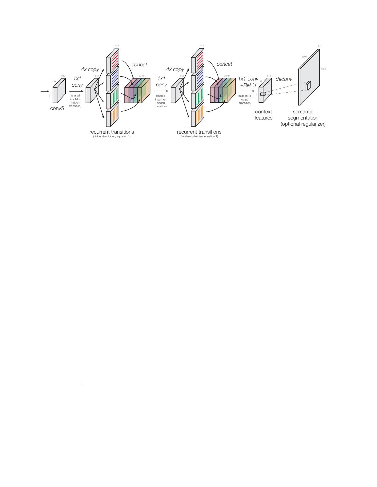
Figure 3. Four-directional IRNN architecture. We use “IRNN” units [21] which are RNNs with ReLU recurrent transitions, initialized

to the identity. All transitions to/from the hidden state are computed with 1x1 convolutions, which allows us to compute the recurrence

more efﬁciently (Eq. 1). When computing the context features, the spatial resolution remains the same throughout (same as conv5). The

semantic segmentation regularizer has a 16x higher resolution; it is optional and gives a small improvement of around +1 mAP point.

3. Architecture: Inside-Outside Net (ION)

In this section we describe ION, a detector with an im-

proved descriptor both inside and outside the ROI. An im-

age is processed by a single deep ConvNet, and the con-

volutional feature maps at each stage of the ConvNet are

stored in memory. At the top of the network, a 2x stacked

4-directional IRNN (explained later) computes context fea-

tures that describe the image both globally and locally. The

context features have the same dimensions as “conv5.” This

is done once per image. In addition, we have thousands

of proposal regions (ROIs) that might contain objects. For

each ROI, we extract a ﬁxed-length feature descriptor from

several layers (“conv3”, “conv4”, “conv5”, and “context

features”). The descriptors are L2-normalized, concate-

nated, re-scaled, and dimension-reduced (1x1 convolution)

to produce a ﬁxed-length feature descriptor for each pro-

posal of size 512x7x7. Two fully-connected (FC) layers

process each descriptor and produce two outputs: a one-of-

K object class prediction (“softmax”), and an adjustment to

the proposal region’s bounding box (“bbox”).

The rest of this section explains the details of ION and

motivates why we chose this particular architecture.

3.1. Pooling from multiple layers

Recent successful detectors such as Fast R-CNN, Faster

R-CNN [30], and SPPnet, all pool from the last convolu-

tional layer (“conv5

3”) in VGG16 [35]. In order to extend

this to multiple layers, we must consider issues of dimen-

sionality and amplitude.

Since we know that pre-training on ImageNet is im-

portant to achieve state-of-the-art performance [1], and

we would like to use the previously trained VGG16 net-

work [35], it is important to preserve the existing layer

shapes. Therefore, if we want to pool out of more layers,

the ﬁnal feature must also be shape 512x7x7 so that it is

the correct shape to feed into the ﬁrst fully-connected layer

(fc6). In addition to matching the original shape, we must

also match the original activation amplitudes, so that we can

feed our feature into fc6.

To match the required 512x7x7 shape, we concatenate

each pooled feature along the channel axis and reduce the

dimension with a 1x1 convolution. To match the original

amplitudes, we L2 normalize each pooled ROI and re-scale

back up by an empirically determined scale. Our experi-

ments use a “scale layer” with a learnable per-channel scale

initialized to 1000 (measured on the training set). We later

show in Section 5.2 that a ﬁxed scale works just as well.

As a ﬁnal note, as more features are concatenated to-

gether, we need to correspondingly decrease the initial

weight magnitudes of the 1x1 convolution, so we use

“Xavier” initialization [36].

3.2. Context features with IRNNs

Our architecture for computing context features in ION

is shown in more detail in Figure 3. On top of the last convo-

lutional layer (conv5), we place RNNs that move laterally

across the image. Traditionally, an RNN moves left-to-right

along a sequence, consuming an input at every step, updat-

ing its hidden state, and producing an output. We extend

this to two dimensions by placing an RNN along each row

and along each column of the image. We have four RNNs in

total that move in the cardinal directions: right, left, down,

up. The RNNs sit on top of conv5 and produce an output

with the same shape as conv5.

There are many possible forms of recurrent neural net-

works that we could use: gated recurrent units (GRU) [4],

long short-term memory (LSTM) [14], and plain tanh re-

current neural networks. In this paper, we explore RNNs

composed of rectiﬁed linear units (ReLU). Le et al. [21]

剩余10页未读，继续阅读

Fate_LordMasterKing

粉丝: 0
资源: 6

利用跳跃池化与RNN在场景中精确检测物体

CNN和RNN进行异常行为检测含数据集-内含源码和说明书(可自己修改).zip

Python-本项目基于yolo3与crnn实现中文自然场景文字检测及识别

text-classification-cnn-rnn-master_RNN_CNN_

RNN的应用和使用场景

在不同场景下的不同位置识别物体

文献以不同的方式结合了卷积神经网络(CNN)和递归神经网络(RNN)对工业时间序列数据进行异常检测，在实际工业场景中取得了良好的检测效果。

cnn和rnn有什么区别

cnn 和 rnn 的应用领域

如何同时使用Transformer和RNN

rnn有没有用到卷积层池化层全连接层

最新资源