20% 40% 60% 80% 100%
Percent of Training Epochs
0.00
0.01
0.02
0.03
0.04
0.05
0.06
0.07
1
d
||
B
||
CIFAR10
IWSLT14
20% 40% 60% 80% 100%
Percent of Training Epochs
0
1
2
3
4
5
6
1
d
||
2 2
B
||
CIFAR10
IWSLT14
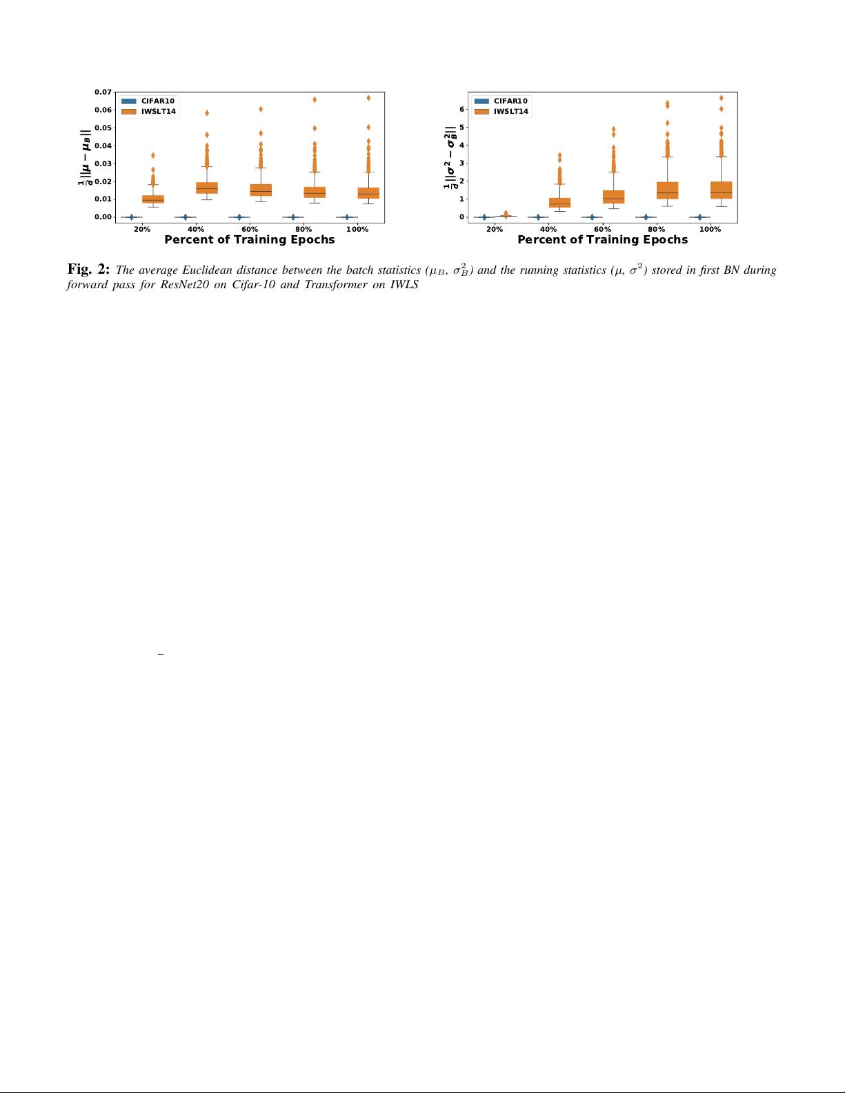
Fig. 2:
The average Euclidean distance between the batch statistics (
µ
B
,
σ
2
B
) and the running statistics (
µ
,
σ
2
) stored in first BN during
forward pass for ResNet20 on Cifar-10 and Transformer on IWLST14. We can clearly see that the ResNet20 statistics have orders of
magnitude smaller variation than the running statistics throughout training. However, the corresponding statistics in Transformer
BN
exhibit
very high variance with extreme outliers. This is true both for the mean (shown in left) as well as variance (shown in right). This is one of
the contributing factors to the low performance of BN in transformers.
This is a significant performance degradation, and
it stems from instabilities associated with the above
four batch statistics. To analyze this, we studied the
batch statistics using the standard setting of ResNet20
on Cifar-10 and Transformer
BN
on IWSLT14 (using a
standard batch size of 128 and tokens of 4K, respectively).
In the first experiment, we probed the fluctuations
between batch statistics,
µ
B
/
σ
B
, and the corresponding
BN running statistics,
µ
/
σ
, throughout training. This is
shown for the first BN layer of ResNet20 on Cifar-10
and Transformer
BN
on IWSLT14 in Figure 2. Here, the
y-axis shows the average Euclidean distance between
batch statistics (
µ
B
,
σ
B
) and the running statistics
(
µ
,
σ
), and the x-axis is different epochs of training,
where we define the average Euclidean distance as
distpµ
B
, µq “
1
d
}µ
B
´ µ}.
The first observation is that Transformer
BN
shows
significantly larger distances between the batch statistics
and the running statistics than ResNet20 on Cifar-10,
which exhibits close to zero fluctuations. Importantly,
this distance between
σ
B
and
σ
significantly increases
throughout training, but with extreme outliers. During
inference, we have to use the running statistics. However,
such large fluctuations would lead to a large inconsistency
between statistics of the testing data and the BN’s
running statistics.
The second observation comes from probing the norm
of
g
µ
and
g
σ
2
defined in Eq. 3, which contribute to
the gradient backpropagation of input. These results
are shown in Figure 3, where we report the norm of
these two parameters for ResNet20 and Transformer
BN
.
For Transformer
BN
, we can see very large outliers,
that actually persist throughout training. This is in
contrast to ResNet20, for which the outliers vanish as
training proceeds.
IV. POWER NORMALIZATION
Based on our empirical observations, we propose
Power Normalization (PN), which effectively resolves
the performance degradation of BN. This is achieved
by incorporating the following two changes to BN.
First, instead of enforcing unit variance, we enforce
unit quadratic mean for the activations. The reason
for this is that we find that enforcing zero-mean and
unit variance in BN is detrimental due to the large
variations in the mean, as discussed in the previous
section. However, we observe that unlike mean/variance,
the unit quadratic mean is significantly more stable for
transformers. Second, we incorporate running statistics
for the quadratic mean of the signal, and we incorporate
an approximate backpropagation method to compute the
corresponding gradient. We find that the combination of
these two changes leads to a significantly more effective
normalization, with results that exceed LN, even when
the same training hyper-parameters are used. Below we
discuss each of these two components.
A. Relaxing Zero-Mean and Enforcing Quadratic Mean
Here, we describe the first modification in PN. As
shown in Figure 2 and 3,
µ
B
and
g
µ
exhibit significant
number of large outliers, which leads to inconsistencies
between training and inference statistics. We first address
this by relaxing the zero-mean normalization, and we use
the quadratic mean of the signal, instead of its variance.
The quadratic mean exhibits orders of magnitude smaller
fluctuations, as shown in Figure 4. We refer to this
4


