OPTIMIZING SPATIAL FILTERS FOR ROBUST EEG SINGLE-TRIAL ANALYSIS 3
central
sulcus
motor
sensory
O
P
T
F
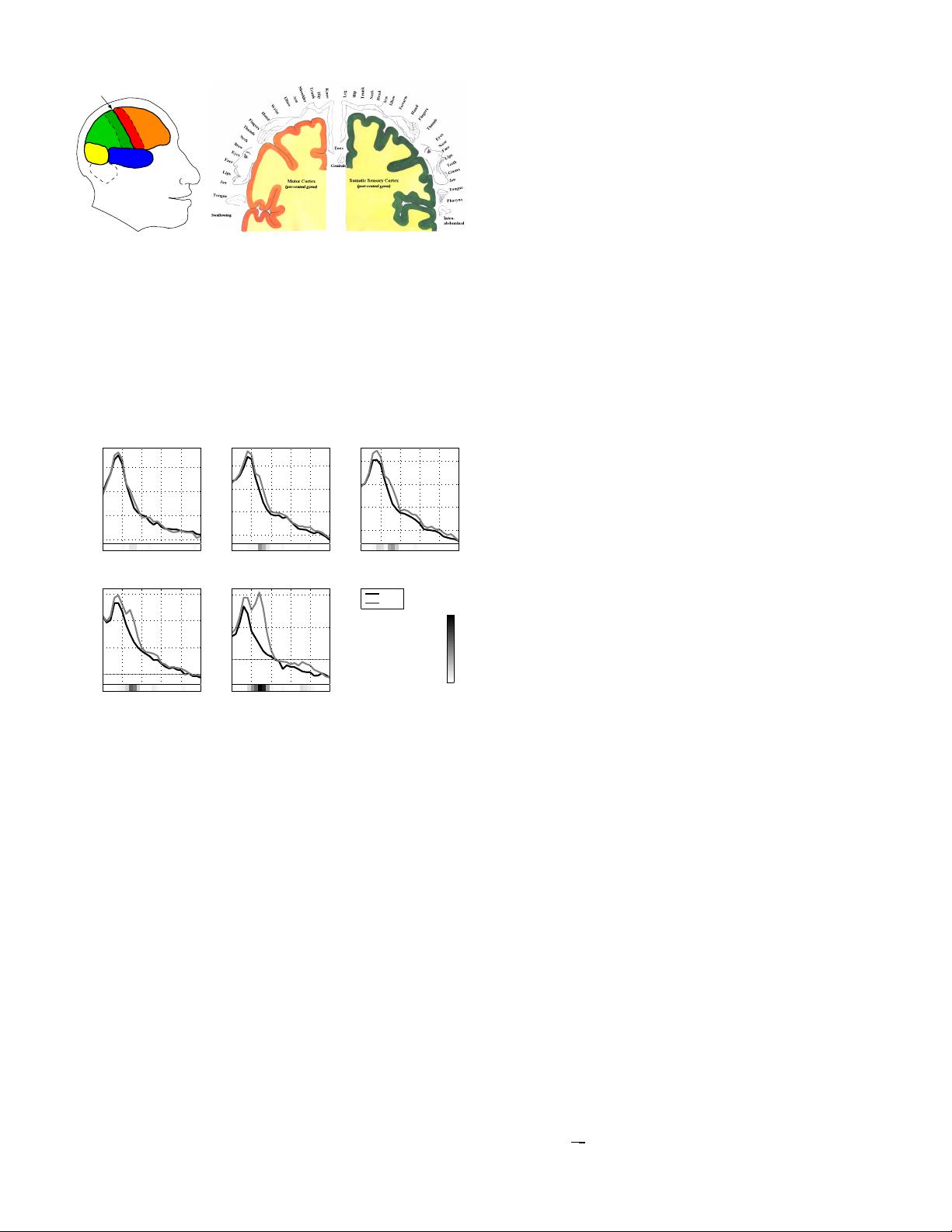
Fig. 3. Left. Lobes of the brain: Frontal, Parietal, Occipital,
and Temporal (named after the bones of the skull beneath which
they are located). The central sulcus separates the frontal and
parietal lobe. Right. Geometric mapping between body parts and
motor/somatosensory cortex. The motor cortex and the somatosensory
cortex are shown at the left and right part of the figure, respectively.
Note, that in each hemisphere there is one motor area (frontal to the
central sulcus) and one sensori area (posterior to the central sulcus).
The part which is not shown can be obtained by mirroring the figure
folded at the center.
5 10 15 20 25 30
15
20
25
30
[Hz]
[dB]
raw: CP4
5 10 15 20 25 30
10
15
20
25
[Hz]
[dB]
bipolar: FC4−CP4
5 10 15 20 25 30
10
15
20
25
[Hz]
[dB]
CAR: CP4
5 10 15 20 25 30
0
5
10
15
[Hz]
[dB]
Laplace: CP4
5 10 15 20 25 30
0
5
10
[Hz]
[dB]
CSP
left
right
0
0.2
0.4
0.6
r
2
Fig. 4. Spectra of left vs. right hand motor imagery. All plots are
calculated from the same dataset but using different spatial filters.
The discrimination between the two conditions is quantified by the
r
2
-value. CAR stands for common average reference.
to the specific characteristics of each user ([19], [2], [7]). For
the latter data-driven approaches to calculate subject-specific
spatial filters have proven to be useful.
As a demonstration of the importance of spatial filters, Fig. 4
shows spectra of left vs. right hand motor imagery at the right
hemispherical sensorimotor cortex. All plots are computed
from the same data but using different spatial filters. While
the raw channel only shows a peak around 9 Hz that provides
almost no discrimination between the two conditions, the
bipolar and the common average reference filter can improve
the discrimination slightly. However the Laplace filter and even
more the CSP filter reveal a second spectral peak around 12 Hz
with strong discriminative power. By further investigations
the spatial origin of the non-discriminative peak could be
traced back to the visual cortex, while the discriminative
peak originates from sensorimotor rhythms. Note that in many
subjects the frequency ranges of visual and sensorimotor
rhythms overlap or completely coincide.
III. METHODS
A. General framework
Here we overview the classifier we use. Let X ∈ R
C×T
be a short segment of EEG signal
2
, which corresponds to a
trial of imaginary movement; C is the number of channels
and T is the number of sampled time points in a trial. A
classifier is a function that predicts the label of a given trial
X. For simplicity let us focus on the binary classification
e.g., classification between imagined movement of left and
right hand. The classifier outputs a real value whose sign is
interpreted as the predicted class. The classifier is written as
follows:
f (X; {w
j
}
J
j=1
, {β
j
}
J
j=0
) =
J
∑
j=1
β
j
log
w
>
j
XX
>
w
j
+ β
0
. (2)
The classifier first projects the signal by J spatial filters
{w
j
}
J
j=1
∈ R
C×J
; next it takes the logarithm of the power of
the projected signal; finally it linearly combines these J di-
mensional features and adds a bias β
0
. In fact, each projection
captures different spatial localization; the modulation of the
rhythmic activity is captured by the log-power of the band-pass
filtered signal. Note that various extensions are possible (see
Sec. V-D). A different experimental paradigm might require
the use of nonlinear methods of feature extraction and classifi-
cation respectively [33]. Direct minimization of discriminative
criterion [17] and marginalization of the classifier weight [22]
are suggested. On the other hand, methods that are linear in
the second order statistics X X
>
, i.e., Eq. (2) without the log,
are discussed in [49], [48] and shown to have some good
properties such as convexity.
The coefficients {w
j
}
J
j=1
and {β
j
}
J
j=1
are automatically
determined statistically ([21]) from the training examples i.e.,
the pairs of trials and labels {X
i
,y
i
}
n
i=1
we collect in the
calibration phase; the label y ∈ {+1,−1} corresponds to, e.g.,
imaginary movement of left and right hand, respectively, and
n is the number of trials.
We use Common Spatial Pattern (CSP) [18], [27] to deter-
mine the spatial filter coefficients {w
j
}
J
j=1
. In the following,
we discuss the method in detail and present some recent
extensions. The linear weights {β
j
}
J
j=1
are determined by
Fisher’s linear discriminant analysis (LDA).
B. Introduction to Common Spatial Patterns Analysis
Common Spatial Pattern ([18], [27]) is a technique to
analyze multi-channel data based on recordings from two
classes (conditions). CSP yields a data-driven supervised de-
composition of the signal parameterized by a matrix W ∈R
C×C
(C being the number of channels) that projects the signal
x(t) ∈ R
C
in the original sensor space to x
CSP
(t) ∈ R
C
, which
lives in the surrogate sensor space, as follows:
x
CSP
(t) = W
>
x(t).
2
In the following, we also use the notation x(t) ∈R
C
to denote EEG signal
at a specific time point t; thus X is a column concatenation of x(t)’s as
X = [x(t),x(t +1), . . .,x(t + T −1)] for some t but the time index t is omitted.
For simplicity we assume that X is already band-pass filtered, centered and
scaled i.e., X =
1
√
T
X
band−pass
(I
T
−1
T
1
>
T
), where I
T
denotes T ×T identity
matrix and 1
T
denotes a T-dimensional vector with all one.


