深度学习架构在人工智能中的应用

5星 · 超过95%的资源需积分: 9 188 浏览量更新于2024-07-25 2 收藏 940KB PDF 举报

“Learning Deep Architectures for AI - Yoshua Bengio - Foundations and Trends in Machine Learning” 在人工智能领域，深度学习已经成为一种强大的工具，特别是在理解和解决复杂的功能表示方面，比如视觉、语言和其他高级任务。《Learning Deep Architectures for AI》这篇论文由Yoshua Bengio撰写，探讨了构建和学习深度架构的关键概念和理论。深度架构是由多层非线性操作组成的，如具有多个隐藏层的神经网络或复杂的命题公式，它们重用许多子公式。这些层次结构的设计目的是模拟人类大脑的分层信息处理机制，从而更好地捕捉数据中的抽象特征。尽管深度学习模型的参数空间极其庞大，使得学习过程极具挑战性，但近年来已经开发出如深度信念网络（Deep Belief Networks, DBNs）等学习算法，成功地解决了这一问题，并在某些领域超越了传统方法，创下了新的性能纪录。论文深入讨论了设计深度学习算法的动机和原则，特别是利用单层无监督学习模型（如受限玻尔兹曼机，Restricted Boltzmann Machines, RBMs）作为构建块的方法。无监督学习在预训练阶段可以帮助初始化深层网络的权重，这可以极大地提高后续的监督学习阶段的效率和性能。预训练与微调相结合的策略，已经成为深度学习中一个关键步骤，它能够有效地避免过拟合，同时提升模型的泛化能力。此外，论文还探讨了深度学习中的其他重要技术，如反向传播（Backpropagation）在优化过程中的作用，以及如何通过正则化和dropout策略来控制模型的复杂性，防止过拟合。在实际应用中，这些技术对于构建能够处理大量数据并从中学习复杂模式的系统至关重要。深度学习不仅限于神经网络，还包括其他类型的深度模型，如卷积神经网络（Convolutional Neural Networks, CNNs）在图像识别和处理中的应用，以及递归神经网络（Recurrent Neural Networks, RNNs）在自然语言处理中的使用。这些模型能够处理序列数据，捕获时间依赖性，并在序列预测任务中展现出卓越的性能。《Learning Deep Architectures for AI》这篇论文为理解深度学习的基本原理和实践提供了全面的视角，强调了深度架构在AI领域的潜力，并为研究者和从业者提供了探索和改进深度学习模型的指导框架。随着计算能力的增强和大数据集的可用性，深度学习将继续推动人工智能的边界，促进更加智能和自主的系统的发展。

In the above equation, f(x) could be for example the discriminant function of a classiﬁer, or the output of a

regression predictor.

A kernel is local when K(x, x

) > ρ is true only for x in some connected region around x

(for some

threshold ρ). The size of that region can usually be controlled by a hyper-parameter of the kernel function.

An example of local kernel is the Gaussian kernel K(x, x

) = e

−||x−x

/σ

, where σ controls the size of

the region around x

. We can see the Gaussian kernel as computing a soft conjunction, because it can be

written as a product of one-dimensional conditions: K(u, v) =

−(u

−v

)

/σ

. If |u

− v

|/σ is small

for all dimensions j, then the pattern matches and K(u, v) is large. If |u

− v

|/σ is large for a single j,

then there is no match and K(u, v) is small.

Well-known examples of kernel machines include Support Vector Machines (SVMs) (Boser, Guyon, &

Vapnik, 1992; Cortes & Vapnik, 1995) and Gaussian processes (Williams & Rasmussen, 1996)

for classiﬁ-

cation and regression, but also classical non-parametric learning algorithms for classiﬁcation, regression and

density estimation, such as the k-nearest neighbor algorithm, Nadaraya-Watson or Parzen windows density

and regression estimators, etc. Below, we discuss manifold learning algorithms such as Isomap and LLE that

can also be seen as local kernel machines, as well as related semi-supervised learning algorithms also based

on the construction of a neighborhood graph (with one node per example and arcs between neighboring

examples).

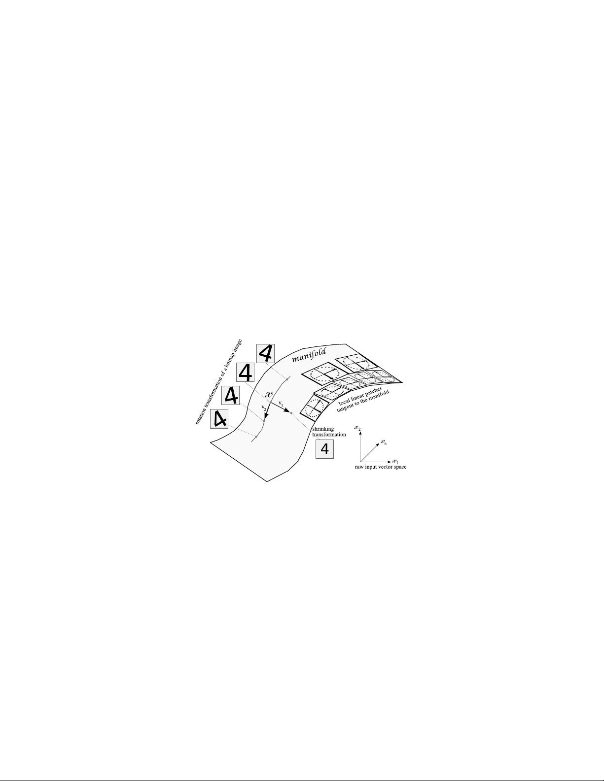
Kernel machines with a local kernel yield generalization by exploiting what could be called the smooth-

ness prior: the assumption that the target function is smooth or can be well approximated with a smooth

function. For example, in supervised learning, if we have the training example (x

, y

), then it makes sense

to construct a predictor f (x) which will output something close to y

when x is close to x

. Note how this

prior requires deﬁning a notion of proximity in input space. This is a useful prior, but one of the claims

made in Bengio, Delalleau, and Le Roux (2006) and Bengio and LeCun (2007) is that such a prior is often

insufﬁcient to generalize when the target function is highly-varying in input space.

The limitations of a ﬁxed generic kernel such as the Gaussian kernel have motivated a lot of research in

designing kernels based on prior knowledge about the task (Jaakkola & Haussler, 1998; Sch¨olkopf, Mika,

Burges, Knirsch, M¨uller, R¨atsch, & Smola, 1999b; G¨artner, 2003; Cortes, Haffner, & Mohri, 2004). How-

ever, if we lack sufﬁcient prior knowledge for designing an appropriate kernel, can we learn it? This question

also motivated much research (Lanckriet, Cristianini, Bartlett, El Gahoui, & Jordan, 2002; Wang & Chan,

2002; Cristianini, Shawe-Taylor, Elisseeff, & Kandola, 2002), and deep architectures can be viewed as a

promising development in this direction. It has been shown that a Gaussian Process kernel machine can

be improved using a Deep Belief Network to learn a feature space (Salakhutdinov & Hinton, 2008): after

training the Deep Belief Network, its parameters are used to initialize a deterministic non-linear transfor-

mation (a multi-layer neural network) that computes a feature vector (a new feature space for the data), and

that transformation can be tuned to minimize the prediction error made by the Gaussian process, using a

gradient-based optimization. The feature space can be seen as a learned representation of the data. Good

representations bring close to each other examples which share abstract characteristics that are relevant fac-

tors of variation of the data distribution. Learning algorithms for deep architectures can be seen as ways to

learn a good feature space for kernel machines.

Consider one direction v in which a target function f (what the learner should ideally capture) goes

up and down (i.e. as α increases, f (x + αv) − b crosses 0, becomes positive, then negative, positive,

then negative, etc.), in a series of “bumps”. Following Schmitt (2002), Bengio et al. (2006), Bengio and

LeCun (2007) show that for kernel machines with a Gaussian kernel, the required number of examples

grows linearly with the number of bumps in the target function to be learned. They also show that for a

maximally varying function such as the parity function, the number of examples necessary to achieve some

error rate with a Gaussian kernel machine is exponential in the input dimension. For a learner that only relies

on the prior that the target function is locally smooth (e.g. Gaussian kernel machines), learning a function

with many sign changes in one direction is fundamentally difﬁcult (requiring a large VC-dimension, and a

In the Gaussian Process case, as in kernel regression, f(x) in eq. 2 is the conditional expectation of the target variable Y to predict,

given the input x.

correspondingly large number of examples). However, learning could work with other classes of functions

in which the pattern of variations is captured compactly (a trivial example is when the variations are periodic

and the class of functions includes periodic functions that approximately match).

For complex tasks in high dimension, the complexity of the decision surface could quickly make learning

impractical when using a local kernel method. It could also be argued that if the curve has many variations

and these variations are not related to each other through an underlying regularity, then no learning algorithm

will do much better than estimators that are local in input space. However, it might be worth looking for

more compact representations of these variations, because if one could be found, it would be likely to lead to

better generalization, especially for variations not seen in the training set. Of course this could only happen

if there were underlying regularities to be captured in the target function; we expect this property to hold in

AI tasks.

Estimators that are local in input space are found not only in supervised learning algorithms such as those

discussed above, but also in unsupervised and semi-supervised learning algorithms, e.g. Locally Linear

Embedding (Roweis & Saul, 2000), Isomap (Tenenbaum, de Silva, & Langford, 2000), kernel Principal

Component Analysis (Sch¨olkopf, Smola, & M¨uller, 1998) (or kernel PCA) Laplacian Eigenmaps (Belkin &

Niyogi, 2003), Manifold Charting (Brand, 2003), spectral clustering algorithms (Weiss, 1999), and kernel-

based non-parametric semi-supervised algorithms (Zhu, Ghahramani, & Lafferty, 2003; Zhou, Bousquet,

Navin Lal, Weston, & Sch¨olkopf, 2004; Belkin, Matveeva, & Niyogi, 2004; Delalleau, Bengio, & Le Roux,

2005). Most of these unsupervised and semi-supervised algorithms rely on the neighborhood graph: a graph

with one node per example and arcs between near neighbors. With these algorithms, one can get a geometric

intuition of what they are doing, as well as how being local estimators can hinder them. This is illustrated

with the example in Figure 4 in the case of manifold learning. Here again, it was found that in order to cover

the many possible variations in the function to be learned, one needs a number of examples proportional to

the number of variations to be covered (Bengio, Monperrus, & Larochelle, 2006).

Figure 4: The set of images associated with the same object class forms a manifold or a set of disjoint

manifolds, i.e. regions of lower dimension than the original space of images. By rotating or shrinking, e.g.,

a digit 4, we get other images of the same class, i.e. on the same manifold. Since the manifold is locally

smooth, it can in principle be approximated locally by linear patches, each being tangent to the manifold.

Unfortunately, if the manifold is highly curved, the patches are required to be small, and exponentially many

might be needed with respect to manifold dimension. Graph graciously provided by Pascal Vincent.

Finally let us consider the case of semi-supervised learning algorithms based on the neighborhood

graph (Zhu et al., 2003; Zhou et al., 2004; Belkin et al., 2004; Delalleau et al., 2005). These algorithms

partition the neighborhood graph in regions of constant label. It can be shown that the number of regions

with constant label cannot be greater than the number of labeled examples (Bengio et al., 2006). Hence one

needs at least as many labeled examples as there are variations of interest for the classiﬁcation. This can be

prohibitive if the decision surface of interest has a very large number of variations.

Decision trees (Breiman, Friedman, Olshen, & Stone, 1984) are among the best studied learning algo-

rithms. Because they can focus on speciﬁc subsets of input variables, at ﬁrst blush they seem non-local.

However, they are also local estimators in the sense of relying on a partition of the input space and using

separate parameters for each region (Bengio, Delalleau, & Simard, 2009), with each region associated with

a leaf of the decision tree. This means that they also suffer from the limitation discussed above for other

non-parametric learning algorithms: they need at least as many training examples as there are variations

of interest in the target function, and they cannot generalize to new variations not covered in the training

set. Theoretical analysis (Bengio et al., 2009) shows speciﬁc classes of functions for which the number of

training examples necessary to achieve a given error rate is exponential in the input dimension. This analysis

is built along lines similar to ideas exploited previously in the computational complexity literature (Cucker

& Grigoriev, 1999). These results are also in line with previous empirical results (P´erez & Rendell, 1996;

Vilalta, Blix, & Rendell, 1997) showing that the generalization performance of decision trees degrades when

the number of variations in the target function increases.

Ensembles of trees (like boosted trees (Freund & Schapire, 1996), and forests (Ho, 1995; Breiman,

2001)) are more powerful than a single tree. They add a third level to the architecture which allows the

model to discriminate among a number of regions exponential in the number of parameters (Bengio et al.,

2009). As illustrated in Figure 5, they implicitly form a distributed representation (a notion discussed further

in Section 3.2) with the output of all the trees in the forest. Each tree in an ensemble can be associated with

a discrete symbol identifying the leaf/region in which the input example falls for that tree. The identity

of the leaf node in which the input pattern is associated for each tree forms a tuple that is a very rich

description of the input pattern: it can represent a very large number of possible patterns, because the number

of intersections of the leaf regions associated with the n trees can be exponential in n.

3.2 Learning Distributed Representations

In Section 1.2, we argued that deep architectures call for making choices about the kind of representation

at the interface between levels of the system, and we introduced the basic notion of local representation

(discussed further in the previous section), of distributed representation, and of sparse distributed repre-

sentation. The idea of distributed representation is an old idea in machine learning and neural networks

research (Hinton, 1986; Rumelhart et al., 1986a; Miikkulainen & Dyer, 1991; Bengio, Ducharme, & Vin-

cent, 2001; Schwenk & Gauvain, 2002), and it may be of help in dealing with the curse of dimensionality

and the limitations of local generalization. A cartoon local representation for integers i ∈ {1, 2, . . . , N} is a

vector r(i) of N bits with a single 1 and N − 1 zeros, i.e. with j-th element r

(i) = 1

i=j

, called the one-hot

representation of i. A distributed representation for the same integer could be a vector of log

N bits, which

is a much more compact way to represent i. For the same number of possible conﬁgurations, a distributed

representation can potentially be exponentially more compact than a very local one. Introducing the notion

of sparsity (e.g. encouraging many units to take the value 0) allows for representations that are in between

being fully local (i.e. maximally sparse) and non-sparse (i.e. dense) distributed representations. Neurons

in the cortex are believed to have a distributed and sparse representation (Olshausen & Field, 1997), with

around 1-4% of the neurons active at any one time (Attwell & Laughlin, 2001; Lennie, 2003). In practice,

we often take advantage of representations which are continuous-valued, which increases their expressive

power. An example of continuous-valued local representation is one where the i-th element varies according

to some distance between the input and a prototype or region center, as with the Gaussian kernel discussed

in Section 3.1. In a distributed representation the input pattern is represented by a set of features that are not

mutually exclusive, and might even be statistically independent. For example, clustering algorithms do not

build a distributed representation since the clusters are essentially mutually exclusive, whereas Independent

Component Analysis (ICA) (Bell & Sejnowski, 1995; Pearlmutter & Parra, 1996) and Principal Component

Analysis (PCA) (Hotelling, 1933) build a distributed representation.

Consider a discrete distributed representation r(x) for an input pattern x, where r

(x) ∈ {1, . . . M},

Partition 1

C3=0

C1=1

C2=1

C3=0

C1=0

C2=0

C3=0

C1=0

C2=1

C3=0

C1=1

C2=1

C3=1

C1=1

C2=0

C3=1

C1=1

C2=1

C3=1

C1=0

Partition 3

Partition 2

C2=0

Figure 5: Whereas a single decision tree (here just a 2-way partition) can discriminate among a number of

regions linear in the number of parameters (leaves), an ensemble of trees (left) can discriminate among a

number of regions exponential in the number of trees, i.e. exponential in the total number of parameters (at

least as long as the number of trees does not exceed the number of inputs, which is not quite the case here).

Each distinguishable region is associated with one of the leaves of each tree (here there are 3 2-way trees,

each deﬁning 2 regions, for a total of 7 regions). This is equivalent to a multi-clustering, here 3 clusterings

each associated with 2 regions. A binomial RBM with 3 hidden units (right) is a multi-clustering with 2

linearly separated regions per partition (each associated with one of the three binomial hidden units). A

multi-clustering is therefore a distributed representation of the input pattern.

i ∈ {1, . . . , N}. Each r

(x) can be seen as a classiﬁcation of x into M classes. As illustrated in Figure 5

(with M = 2), each r

(x) partitions the x-space in M regions, but the different partitions can be combined

to give rise to a potentially exponential number of possible intersection regions in x-space, corresponding

to different conﬁgurations of r(x). Note that when representing a particular input distribution, some con-

ﬁgurations may be impossible because they are incompatible. For example, in language modeling, a local

representation of a word could directly encode its identity by an index in the vocabulary table, or equivalently

a one-hot code with as many entries as the vocabulary size. On the other hand, a distributed representation

could represent the word by concatenating in one vector indicators for syntactic features (e.g., distribution

over parts of speech it can have), morphological features (which sufﬁx or preﬁx does it have?), and semantic

features (is it the name of a kind of animal? etc). Like in clustering, we construct discrete classes, but the

potential number of combined classes is huge: we obtain what we call a multi-clustering and that is similar to

the idea of overlapping clusters and partial memberships (Heller & Ghahramani, 2007; Heller, Williamson,

& Ghahramani, 2008) in the sense that cluster memberships are not mutually exclusive. Whereas clustering

forms a single partition and generally involves a heavy loss of information about the input, a multi-clustering

provides a set of separate partitions of the input space. Identifying which region of each partition the input

example belongs to forms a description of the input pattern which might be very rich, possibly not losing

any information. The tuple of symbols specifying which region of each partition the input belongs to can

be seen as a transformation of the input into a new space, where the statistical structure of the data and the

factors of variation in it could be disentangled. This corresponds to the kind of partition of x-space that an

ensemble of trees can represent, as discussed in the previous section. This is also what we would like a deep

architecture to capture, but with multiple levels of representation, the higher levels being more abstract and

representing more complex regions of input space.

In the realm of supervised learning, multi-layer neural networks (Rumelhart et al., 1986a, 1986b) and in

the realm of unsupervised learning, Boltzmann machines (Ackley, Hinton, & Sejnowski, 1985) have been

introduced with the goal of learning distributed internal representations in the hidden layers. Unlike in

the linguistic example above, the objective is to let learning algorithms discover the features that compose

the distributed representation. In a multi-layer neural network with more than one hidden layer, there are

剩余70页未读，继续阅读

机器再学习

粉丝: 80
资源: 25

深度学习架构在人工智能中的应用

深度学习架构：人工智能的基石

深度学习架构的理论与实践

深度学习架构的学习与理论优势

Learning Deep Architectures for AI.pdf

Creating_Brain-Like_Intelligence\Learning deep Architectures for AI

学习AI的深层架构（Yoshua Bengio）Learning Deep Architectures for AI (Yoshua Bengio)

Learning deep architecture for AI

Hands-On Deep Learning Architectures with Python Create deep neu

Deep Learning for Image Processing Applications

Deep_Learning_Architecture_for_AI.pdf

最新资源