EPnP：线性时间复杂度的精确PnP问题解决方案

需积分: 44 8 浏览量更新于2024-09-06 收藏 2.3MB PDF 举报

EPnP（Essential+PointnPose）是一项创新的计算机视觉技术，旨在解决单个相机姿态（即相机的位置和旋转）从三维点到二维投影点对应关系的精确估计问题。相比于现有的算法，EPnP提出了一种非迭代的解决方案，其计算复杂度显著降低，由原来的O(n^5)或O(n^8)降低至线性时间复杂度O(n)，这使得在大规模数据集上处理PnP问题变得更加高效。 EPnP的核心思想是将三维点集表示为四个虚拟控制点的加权和。通过这种方式，问题被简化为在相机坐标系中估计这些控制点的坐标。这个过程可以通过构建一个12x12的矩阵来实现，其元素与点对之间的投影关系有关。通过计算该矩阵的特征向量，并解出少量的二次方程，可以快速找到合适的权重，从而在常数时间内完成控制点坐标的求解。值得注意的是，EPnP不仅适用于平面配置，也能妥善处理非平面场景，显示了其在实际应用中的广泛适用性。即使对于需要最高精度的情况，EPnP的封闭形式解可以作为Gauss-Newton迭代优化的初始猜测，进一步提高了收敛速度和精度。这种方法的优点在于它提供了一个简洁且高效的工具箱，对于需要实时或者大数据量下处理视觉定位和追踪问题的领域，如机器人导航、增强现实和三维重建等，具有革命性的意义。 EPnP是一项重要的贡献，它革新了单视图立体匹配中的PnP问题求解，通过优化计算效率和保持准确性，为计算机视觉研究和实践带来了实质性的提升。它的出现有望推动相关领域的技术进步，并促进更广泛的机器智能应用的发展。

0 50 100 150

0.01

0.02

0.03

0.04

0.05

0.06

0.07

number of points used to estimate pose

computation time (sec)

Clamped DLT

LHM

EPnP

EPnP+LHM

EPnP+Gauss−Newton

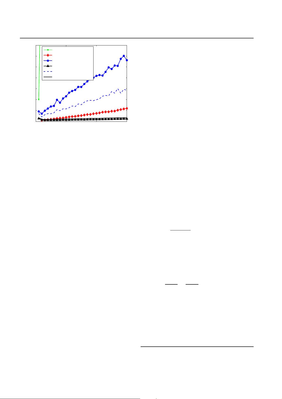
Fig. 2 Comparing computation times of our method against the

state-of-the-art ones introduced in Fig. 1. The computation times

of a MATLAB implementation on a standard PC, are plotted

as a function of the number of correspondences. Our method

is both more accurate—see Fig. 1—and faster than the other

non-iterative ones, especially for large amounts of noise, and is

almost as accurate as the iterative LHM. Furthermore, if maximal

precision is required, the output of our algorithm can be used to

initialize a Gauss-Newton optimization procedure which requires

a negligible amount of additional time.

dinates of the control points in the camera referential,

which can be done in O(n) time by expressing these

coordinates as weighted sum of the eigenvectors of a

12 × 12 matrix and solving a small constant number

of quadratic equations to pick the right weights. Our

approach also extends to planar conﬁgurations, which

cause problems for some methods as discussed in [23,

25], by using three control points instead of four.

In the remainder of the paper, we ﬁrst discuss re-

lated work focusing on accuracy and computational com-

plexity. We then introduce our new formulation and

derive our system of linear and quadratic equations.

Finally, we compare our method against the state-of-

the-art ones using synthetic data and demonstrate it

using real data. This paper is an expanded version of

that in [22], where a ﬁnal Gauss-Newton optimization

is added to the original algorithm. In Section 4 we show

that optimizing over a reduced number of parameters,

the accuracy of the closed-solution proposed in [22] is

considerably improved with almost no additional com-

putational cost.

2 Related Work

There is an immense body of literature on pose estima-

tion from point correspondences and, here, we focus on

non-iterative approaches since our method falls in this

category. In addition, we will also introduce the Lu et

al. [20] iterative method, which yields very good results

and against which we compare our own approach.

Most of the non-iterative approaches, if not all of

them, proceed by ﬁrst estimating the points 3D posi-

tions in the camera coordinate system by solving for

the points depths. It is then easy to retrieve the cam-

era position and orientation as the Euclidean motion

that aligns these positions on the given coordinates in

the world coordinate system [15,3,30].

The P3P case has been extensively studied in the lit-

erature, and many closed form solutions have been pro-

posed such as [6,8,9,11,24]. It typically involves solving

for the roots of an eight-degree polynomial with only

even terms, yielding up to four solutions in general, so

that a fourth point is needed for disambiguation. Fisher

and Bolles [8] reduced the P4P problem to the P3P one

by taking subsets of three points and checking consis-

tency. Similarly, Horaud et al. [13] reduced the P4P

to a 3-line problem. For the 4 and 5 points problem,

Triggs [29] derived a system of quadratic polynomials,

which solves using multiresultant theory. However, as

pointed out in [2], this does not perform well for larger

number of points.

Even if four correspondences are suﬃcient in gen-

eral to estimate the pose, it is nonetheless desirable

to consider larger point sets to introduce redundancy

and reduce the sensitivity to noise. To do so, Quan and

Lan [24] consider triplets of points and for each one

derive four-degree polynomials in the unknown point

depths. The coeﬃcients of these polynomials are then

arranged in a

(n−1)(n−2)

× 5 matrix and singular value

decomposition (SVD) is used to estimate the unknown

depths. This method is repeated for all of the n points

and therefore involves O(n

) operations.

It should be

noted that, even if it is not done in [24], this complex-

ity could be reduced to O(n

) by applying the same

trick as we do when performing the SVD, but even

then, it would remain slower than our method. Ansar

and Daniilidis [2] derive a set of quadratic equations ar-

ranged in a

n(n−1)



n(n+1)



linear system, which,

as formulated in the paper, requires O(n

) operations

to be solved. They show their approach performs better

than [24].

The complexity of the previous two approaches stems

from the fact that quadratic terms are introduced from

the inter-point distances constraints. The linearization

of these equations produces additional parameters, which

increase the complexity of the system. Fiore’s method [7]

avoids the need for these constraints: He initially forms

Following [10], we consider that the SVD for a m × n matrix

can be computed by a O(4m

n +8mn

+9n

) algorithm.

剩余12页未读，继续阅读

白菜888

粉丝: 7
资源: 74

EPnP：线性时间复杂度的精确PnP问题解决方案

EPnP_matlab.rar_EPnP_MATLAB实现pnp_PnP求解_pnp算法matlab_用Matlab做pnp

PNP算法+后方交会算法

EPnP阅读笔记 .pdf

APnP和epnp算法原理的区别是什么

类似于epnp的非迭代的PnP算法有哪些？

pose_estimation_epnp

PnP算法 估计位姿

epnp算法python

简述EPnP算法的大致步骤

epnp算法c语言实现

最新资源

PnP算法估计位姿