多任务压缩感知在无线传感网络中的应用

需积分: 9 96 浏览量更新于2024-07-25 收藏 2.38MB PDF 举报

"这篇论文是关于多任务压缩感知在无线传感网络中的应用，由Shihao Ji、David Dunson和Lawrence Carin撰写并发表在2009年1月的IEEE Transactions on Signal Processing期刊上。该研究探讨了如何利用压缩感知理论在资源有限的情况下高效地获取和恢复多个信号源的信息。" 在压缩感知（Compressive Sensing，CS）的框架下，系统通过N个非适应性测量来构建一个向量v，这个向量用于恢复一个近似信号^u，其原始信号u是一个M维稀疏向量。这里的N远小于M，即测量数量少于信号的维度，这得益于信号在某个M×M基矩阵下的稀疏特性。研究表明，通过合理设计压缩测量过程，可以实现对v到^u的逆变换，且误差ku-u^k2_2具有与最佳自适应变换编码算法相似的渐近性质。大多数早期的研究中，如果存在L组以上的压缩测量数据fv_v_i (i=1;L)，则每组对应的^u_u_i (i=1;L)会独立地逐一恢复。然而，这种方法忽视了不同任务间可能存在的相关性和潜在的协同效应。论文“Multitask Compressive Sensing”引入了多任务的概念，旨在同时处理和恢复多个信号，以提高整体恢复质量和效率。通过将多个信号的恢复问题融合为一个优化问题，可以利用各个任务间的共性信息，从而减少总的测量次数，降低计算复杂度，并可能提高恢复精度。多任务压缩感知的核心是寻找一种方法，能够同时考虑所有信号的稀疏表示，并在测量过程中利用这些共享特征。这通常涉及到使用联合正则化或多元优化技术，例如`1范数正则化，它能有效地鼓励解决方案的稀疏性。通过这种方式，不仅可以减少传感器网络的通信负担，还能在保持重构质量的同时，提高资源利用率。这篇论文在压缩感知领域提出了一种新的多任务处理方法，它挑战了传统的一次一任务恢复策略，强调了在无线传感网络中利用信号间的共性进行高效数据采集和恢复的重要性。这一理论和技术对于优化无线传感器网络的设计，特别是在资源受限的环境下，具有重要的理论价值和实际应用潜力。

94 IEEE TRANSACTIONS ON SIGNAL PROCESSING, VOL. 57, NO. 1, JANUARY 2009

employed for the fast point estimate of the hyperparameters

and in Fig. 1. This yields a computationally efﬁcient multi-

task CS inference algorithm that extends previous research in

the Bayesian CS analysis [10], wherein the Bayesian inversion

was performed one task at a time (single-task learning,

i.e.,

In addition to a hierarchal Bayesian model of multitask CS

and a fast inference algorithm, a modiﬁed sparse linear-regres-

sion model is developed, of interest both for the single-task and

multitask CS settings. As discussed further below, this extension

analytically integrates out the noise-variance term in the regres-

sion model, and it yields improved robustness over the previous

formulation.

The remainder of the paper is structured as follows. In

Section II we introduce a hierarchical Bayesian model for

multitask CS that builds naturally upon previous research

on Bayesian CS [10]; a fast sequential optimization algo-

rithm based on an empirical Bayesian procedure is developed

for inference. In Section III we propose a modiﬁed sparse

linear-regression model by marginalizing the noise variance,

and develop a fast inference algorithm as well. Example results

on multiple datasets are presented in Section IV. A review of

work related to multitask CS is provided in Section V, followed

in Section VI by conclusions and a discussion of future work.

II. H

IERARCHICAL MULTITASK

CS MODELING

A. Bayesian Regression Formulation

Assume that

sets of CS measurements are performed, with

these multiple sensing tasks statistically interrelated, as deﬁned

precisely later. The

sets of measurements are represented as

, where , and in general each

measurement vector

employs a different random pro-

jection matrix

, for . This gener-

alizes the formulation considered in [12]–[15], [17], wherein a

single

is employed across all the tasks. In the context of a

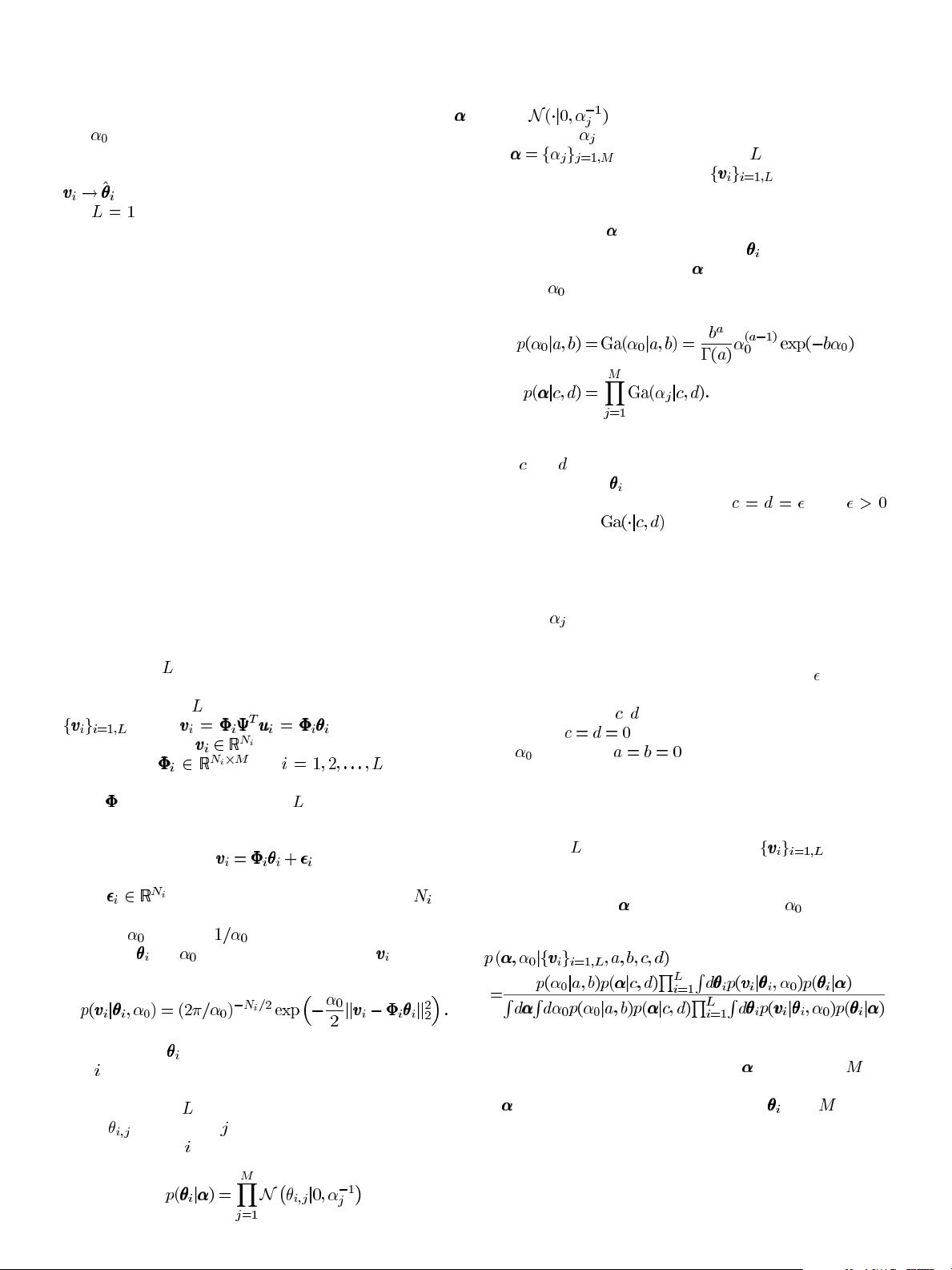
regression analysis, we assume [10]

(2)

where

is a residual error vector, modeled as i.i.d.

draws of a zero-mean Gaussian random variable with unknown

precision

(variance ). The likelihood function for the

parameters

and , based on the observed data , may there-

fore be expressed as

(3)

The parameters

(here, wavelet coefﬁcients) characteristic of

task

are assumed to be drawn from a product of zero-mean

Gaussian distributions that are shared by all tasks, and it is in

this sense that the

tasks are statistically related. Speciﬁcally,

letting

represent the th wavelet (or scaling function) coef-

ﬁcient for CS task

,wehave

(4)

where

is a zero-mean Gaussian density function

with precision

. It is important to note that the hyperparame-

ters

are shared among all tasks, and therefore

the data from all CS measurements

will contribute to

learning the hyperparameters, offering the opportunity to adap-

tively borrow strength from the different measurements to a de-

gree controlled by

To promote sparsity over the weights

, Gamma priors are

placed on the hyperparameters

, and similarly on the noise

precision

(5)

(6)

It has been demonstrated [19] that appropriate choice of param-

eters

and encourages a sparse representation for the coefﬁ-

cients in the vector

, where here this concept is extended to a

multitask CS setting. Typically, when

, with

a small constant, has a large spike concentrated at

zero and a heavy right tail. The spike corresponds to basis func-

tions for which there is essentially no borrowing of information.

Such basis functions characterize components that are idiosyn-

cratic to speciﬁc signals. At the other extreme, basis functions

for which

is in the right tail have coefﬁcients that are shrunk

strongly to zero for all tasks, favoring sparseness, while bor-

rowing information about which basis functions are not impor-

tant for any of the signals in the collection. For small

, there will

be many such basis functions. As a default choice which avoids

subjective choice of

, and leads to computational simpliﬁca-

tions, we set

. For the Gamma prior on the noise preci-

sion

, we also let as a default choice. This choice

corresponds to a commonly-used improper prior expressing a

priori ignorance about plausible values for the residual preci-

sion.

With these parametric deﬁnitions, a graphical model rep-

resentation of multitask CS is illustrated in Fig. 1.

Given the

sets of CS measurements from the

(assumed) statistically related sources, by applying the Bayes’

rule, one may in principle infer a posterior density function on

the hyperparameters

and the noise precision

(7)

where the integral in (7) with respect to

is actually an -di-

mensional integral, with each integral linked to one component

; similarly, each integral with respect to is an -dimen-

sional integral, over all wavelet-coefﬁcient weights. To avoid the

While the sparsity analysis provided here is largely following that of RVM

[19], which is intuitive and conceptual, a more recent and rigorous analysis of

sparse Bayesian learning and its superior performance on sparse representation

can be found at [37], [38]. More relevantly, it is the log-det term of the likelihood

(13) that produces sparsity.

剩余14页未读，继续阅读

ct607

粉丝: 2
资源: 1

多任务压缩感知在无线传感网络中的应用

多任务压缩感知matlab程序

Recommending What Video to Watch Next: A Multitask Ranking System.pdf

Multi-Task Compressive Sensing

WARD方法matlab代码-Distributed-Compressive-Sensing-A-Deep-Learning-Approach

multitask0.2.0

web_multitask

MultiTask.zip

MultiTask分类器

fourier-multitask

simple_multitask

最新资源