is to periodically set the weights of the target network to the current weights of the main network (e.g.
Mnih et al. (2015)) or to use a polyak-averaged
2
(Polyak and Juditsky, 1992) version of the main
network instead (Lillicrap et al., 2015).
2.3 Deep Deterministic Policy Gradients (DDPG)
Deep Deterministic Policy Gradients (DDPG) (Lillicrap et al., 2015) is a model-free RL algorithm
for continuous action spaces. Here we sketch it only informally, see Lillicrap et al. (2015) for more
details. In DDPG we maintain two neural networks: a target policy (also called an actor)
π : S → A
and an action-value function approximator (called the critic)
Q : S × A → R
. The critic’s job is to
approximate the actor’s action-value function Q
π
.
Episodes are generated using a behavioral policy which is a noisy version of the target policy, e.g.
π
b
(s) = π(s) + N (0, 1)
. The critic is trained in a similar way as the Q-function in DQN but the
targets
y
t
are computed using actions outputted by the actor, i.e.
y
t
= r
t
+ γQ(s
t+1
, π(s
t+1
))
.
The actor is trained with mini-batch gradient descent on the loss
L
a
= −E
s
Q(s, π(s))
, where
s
is sampled from the replay buffer. The gradient of
L
a
w.r.t. actor parameters can be computed by
backpropagation through the combined critic and actor networks.
2.4 Universal Value Function Approximators (UVFA)
Universal Value Function Approximators (UVFA) (Schaul et al., 2015a) is an extension of DQN to
the setup where there is more than one goal we may try to achieve. Let
G
be the space of possible
goals. Every goal
g ∈ G
corresponds to some reward function
r
g
: S × A → R
. Every episode starts
with sampling a state-goal pair from some distribution
p(s
0
, g)
. The goal stays fixed for the whole
episode. At every timestep the agent gets as input not only the current state but also the current goal
π : S × G → A
and gets the reward
r
t
= r
g
(s
t
, a
t
)
. The Q-function now depends not only on a
state-action pair but also on a goal
Q
π
(s
t
, a
t
, g) = E[R
t
|s
t
, a
t
, g]
. Schaul et al. (2015a) show that in
this setup it is possible to train an approximator to the Q-function using direct bootstrapping from the
Bellman equation (just like in case of DQN) and that a greedy policy derived from it can generalize
to previously unseen state-action pairs. The extension of this approach to DDPG is straightforward.
3 Hindsight Experience Replay
3.1 A motivating example
Consider a bit-flipping environment with the state space
S = {0, 1}
n
and the action space
A =
{0, 1, . . . , n − 1}
for some integer
n
in which executing the
i
-th action flips the
i
-th bit of the state.
For every episode we sample uniformly an initial state as well as a target state and the policy gets a
reward of −1 as long as it is not in the target state, i.e. r
g
(s, a) = −[s 6= g].
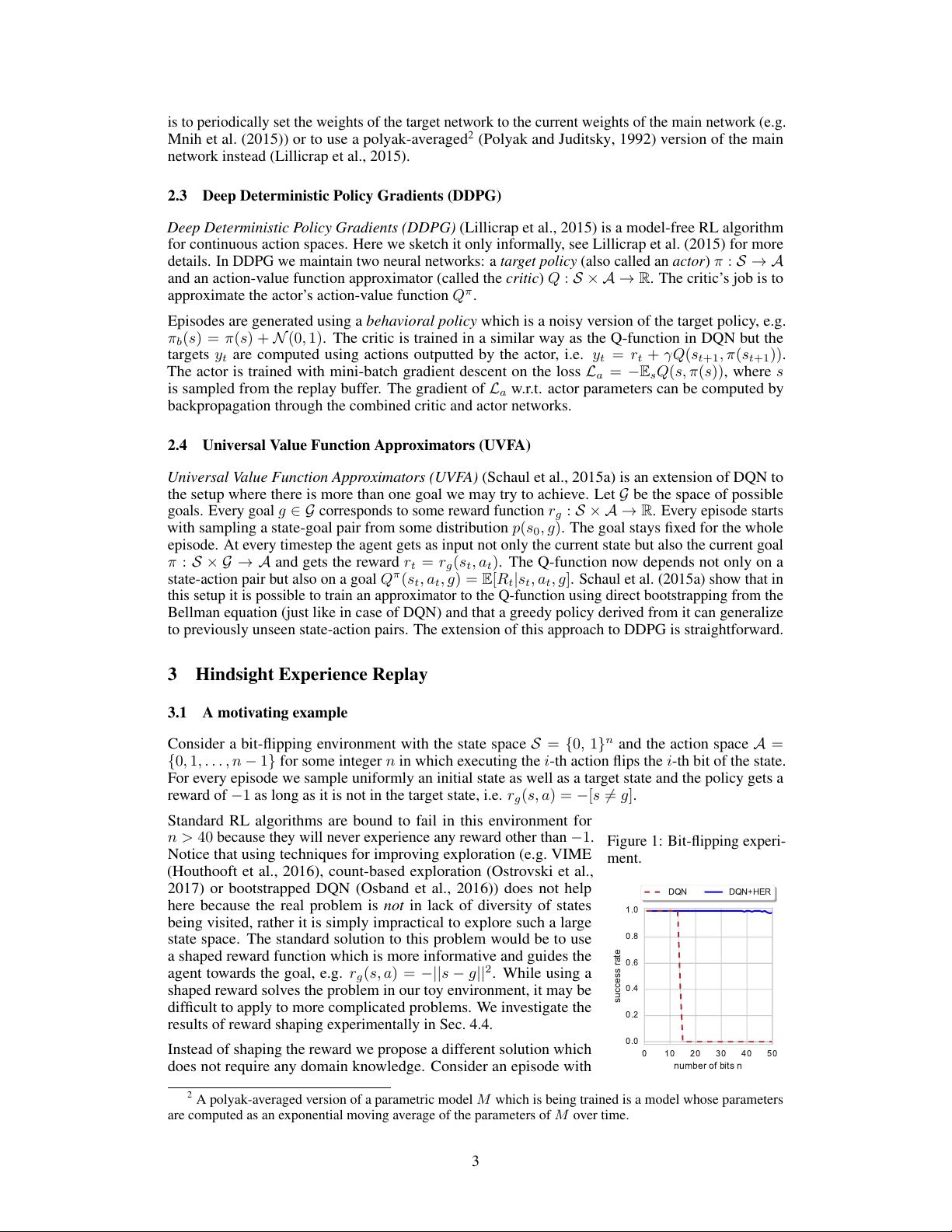
Figure 1: Bit-flipping experi-
ment.
0 10 20 30 40 50
number of bits n
0.0
0.2
0.4
0.6
0.8
1.0
success rate
DQN DQN+HER
Standard RL algorithms are bound to fail in this environment for
n > 40
because they will never experience any reward other than
−1
.
Notice that using techniques for improving exploration (e.g. VIME
(Houthooft et al., 2016), count-based exploration (Ostrovski et al.,
2017) or bootstrapped DQN (Osband et al., 2016)) does not help
here because the real problem is not in lack of diversity of states
being visited, rather it is simply impractical to explore such a large
state space. The standard solution to this problem would be to use
a shaped reward function which is more informative and guides the
agent towards the goal, e.g.
r
g
(s, a) = −||s − g||
2
. While using a
shaped reward solves the problem in our toy environment, it may be
difficult to apply to more complicated problems. We investigate the
results of reward shaping experimentally in Sec. 4.4.
Instead of shaping the reward we propose a different solution which
does not require any domain knowledge. Consider an episode with
2
A polyak-averaged version of a parametric model
M
which is being trained is a model whose parameters
are computed as an exponential moving average of the parameters of M over time.
3


