Fast Semi-Lagrangian方法的多相界面精确追踪

78 浏览量更新于2024-08-30 收藏 667KB PDF 举报

本文探讨了一种快速半拉格朗日轮廓法在多相界面跟踪中的应用，发表于《计算机图形学与可视化交易》(IEEE Transactions on Visualization and Computer Graphics)的2015年9月刊上。作者是李晓生、何小巍、刘雪辉、詹剑杰、刘宝全和吴恩华。该研究论文的创新之处在于提出了一种全新的方法来处理任意数量相界面的追踪，区别于传统的方法。传统界面追踪技术往往依赖于隐式函数或者复杂的后处理步骤，而本文的半拉格朗日方法则采用了一种更直接且高效的策略。它维护一个明确的多边形网格，这个网格由未签名距离函数（Unsigned Distance Function, UDF）和指示函数共同构建，可以直观地表示各相界面的位置。这种方法的优势在于网格结构清晰，易于理解和操作，尤其是在处理动态变化的多相界面时，能够提供稳定的跟踪性能。核心部分介绍了作者们开发的一种有效多相三角化过程，该过程在每次追踪步长中重建表面网格，确保了界面追踪的实时性和准确性。这种半拉格朗日策略结合了拉格朗日追踪的移动性与网格更新的稳定性，使得界面的跟踪不仅精度高，而且具有良好的计算效率。为了实现这一目标，论文详细阐述了算法设计、数据结构的选择以及优化的计算策略，包括如何有效地更新网格，处理界面交点和拓扑变化，以及如何利用并行计算加速处理大规模数据。此外，文中还可能讨论了与现有方法的对比实验结果，证明了新方法在处理复杂多相场景时的优越性，尤其是在实时性和稳定性方面。本篇研究论文为多相界面跟踪领域带来了创新的解决方案，通过半拉格朗日轮廓法，简化了界面表示与追踪的过程，并展示了其在实时图形学和计算机视觉中的实际应用潜力。感兴趣的读者可以在论文的DOI:10.1109/TVCG.2015.2476788找到更多详细信息，这将有助于进一步理解和改进多相流体模拟、图像分割和计算机视觉中的界面追踪技术。

http://www.ieee.org/publications_standards/publications/rights/index.html for more information.

This article has been accepted for publication in a future issue of this journal, but has not been fully edited. Content may change prior to final publication. Citation information: DOI

10.1109/TVCG.2015.2476788, IEEE Transactions on Visualization and Computer Graphics

JOURNAL OF IEEE TRANSACTIONS ON VISUALIZATION AND COMPUTER GRAPHICS, VOL. 13, NO. 9, SEPTEMBER 2015 3

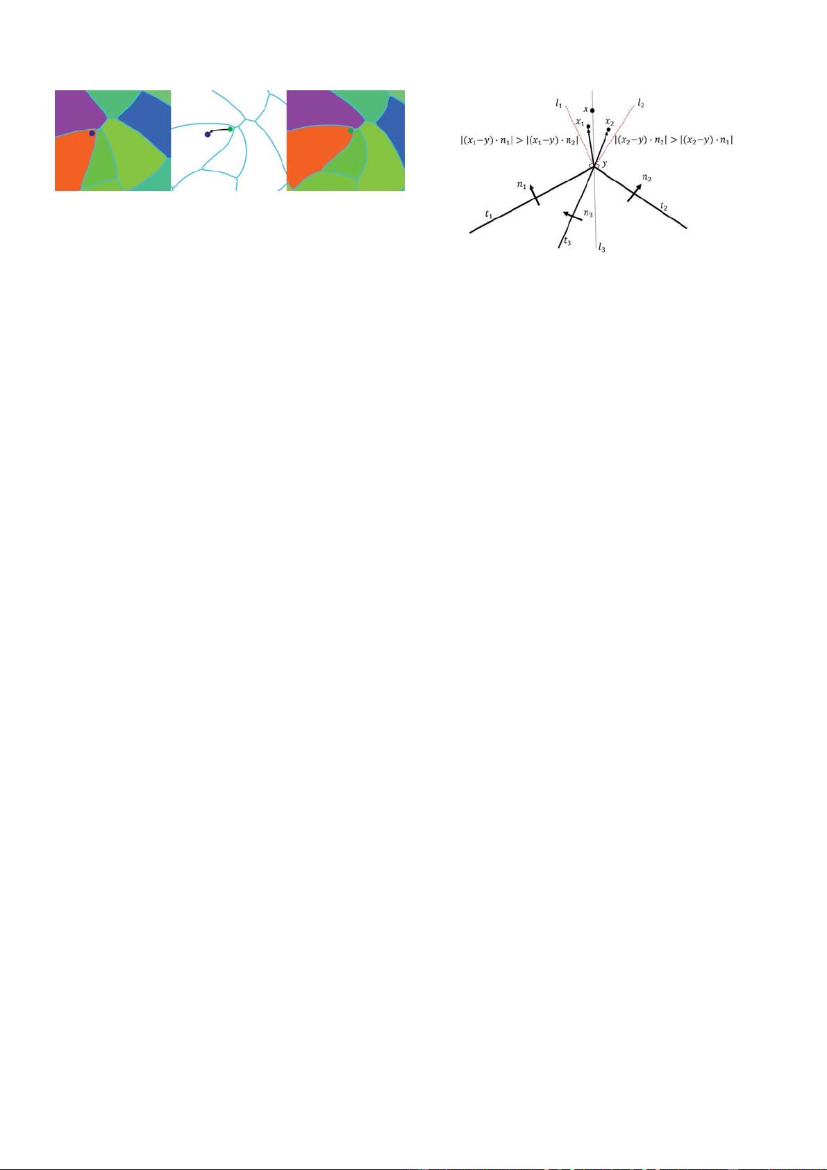
Fig. 1. Update of the distance and indicator functions. Middle: For a point

(green) in space, we trace back a step to ﬁnd its previous position (blue).

Left: Distance and indicator functions are then updated by exact com-

putation from the interface meshes in previous position. Right: Once the

distance and indicator functions are updated, we process to construct a

new interface mesh with the contouring algorithm.

Now we outline our method, formally. Given an N-

phase problem (see Figure 1) equipped with an unsigned

distance function

φ(x), which denotes the distance mea-

sured from

x to the nearest point on the interface, an

indicator function

χ(x), which indicates the phase material,

and an explicit surface mesh, we formulate the tracking

of multiphase interfaces as a contouring problem which

consists of three steps as follows:

1) Update

φ and χ using semi-Lagrangian method. φ

and χ are computed exactly to improve the accura-

cy.

2) Contour

φ and χ to get the new interface meshes.

This is performed with precomputed stencils com-

bined with bisection to get accurate estimations of

intersections and junctions.

3) Redistance

φ and χ.Asφ is most accurate near the

interface, we propagate the values near the interface

to the whole domain to stay in good accuracy.

To advect

φ(x) and χ(x) forward, we use the semi-

Lagrangian method [33] to backtrace the point

x through the

streamline of the velocity ﬁeld

v over a time Δt and assign

the new value with the value at its previous location, i.e.,

φ(x)=φ(x − Δtv), χ(x)=χ(x − Δtv). Here, φ(x − Δtv)

is computed from the explicit surface mesh at the previous

time step, according to [7], and the calculation of

χ(x−Δtv)

requires a special treatment to the representation of the

surface meshes (Section 4). Then, we will reconstruct the

surface meshes from

φ and χ instead of advancing the

meshes forward to avoid the complex remeshing during the

topological changes. The key point of this part is to guar-

antee that the reconstructed surface meshes are watertight

and smooth (Section 5). Finally, since it is expensive to track

multiphase interfaces on a uniform grid, we use an octree

(quadtree in 2D) to store

φ and χ. We only maintain the

ﬁnest cells near the interfaces. As long as the interfaces

are moved, we will adjust the tree’s structure to keep it

balanced. Section 6 gives the details how to build the octree

to well resolve

φ and χ and how to compute φ and χ for the

tree structure efﬁciently.

4DISTANCE AND INDICATOR COMPUTATION

Our multiphase system consists of two parts: an implicit

part, which contains an unsigned distance function

φ as

well as an indicator function

χ, and an explicit part, which

corresponds to the surface meshes. Since the implicit part is

Fig. 2. Indicator computation near a vertex. Only when two neighboring

segments form an angle no less than 180 degrees, the closest point y

can lie on the vertex. In such case, x must lie in the region form by l

and l

. l

and l

are perpendicular to t

and t

respectively. For x

, n

is used to compute the indicator value while n

is used for x

according

to our method. In a non-manifold setting, there can be a third segment

incident on a vertex, say t

. Imagine rotating t

and t

about vertex y to

, we can easily see that |E| = |(x − y ) · n

| is always smaller than that

of t

or t

as |E| keep decreasing to zero when rotating t

and t

to l

until one of them gets over t

. Thus, t

or t

is always used to compute

the indicator value accurately.

similar to the one in VIIM, we only discuss the explicit part

here.

To avoid complicated remeshing operations, we will

always reconstruct the surface meshes from the isocontour

φ(x)=0, from which both the distance function and the

indicator function can be updated accurately. The explicit

representation of the surface mesh is similar to [7], except

that the triangle mesh in our method may be non-manifold

(one edge is shared by more than two triangles) and contains

complex structures such as the T-junctions. Then, it raises

a question: how can we identify a material at any point

x without using a binary inside/outside classiﬁcation of

space? In our implementation, we follow Da and the col-

leagues’ work [34] to assign a unique integer label to each

material and apply different labels to the front and back

of each triangle. Besides, we store an extra normal on each

face of the triangle mesh to facilitate the calculation of the

indicator function. The normal will be always pointing from

a higher material label to a lower one. Now, we will show

how such information is used to divide the entire problem

domain into separate regions of materials.

4.1 Material Identiﬁcation

Since the distance function can be computed according

to [7], we only discuss how to get the indicator function

here. We ﬁrst consider a 2D case. For an arbitrary point

x, we denote its closest point on the curve as y and the

corresponding normal as

n(y), which is assumed to point

from material

A to B. To identify the material label for x,

we ﬁrst calculate the following quantity:

E =(x − y) · n(y) (1)

y lies inside the edge, the material label can easily be

determined from the sign of

E. More speciﬁcally, E > 0

means the point x belongs to material B while E < 0

means it belongs to material A. However, if the point y

lies on the vertex, different values of E can be obtained if we

use the normal deﬁned on different edges. We remove this

ambiguity by choosing the one with the maximum value of

剩余13页未读，继续阅读

weixin_38519387

粉丝: 3
资源: 931

Fast Semi-Lagrangian方法的多相界面精确追踪

testsafetystarteragent

多重分形的matlab代码-Numerical-Lagrangian-Particle-Tracking-Bacteria:拉格朗日数值跟踪细

GSP粉煤气化过程数值模拟：Euler-Lagrangian方法的应用

Multiphase Segmentation on CT Liver Image Using Split-Augmented Lagrangian Projection Method

VSR不变Chern-Simons Lagrangian对光子极化的影响

手性异常，施温格效应，Euler-Heisenberg Lagrangian及其在轴突膨胀中的应用

Lagrangian relaxation-based routing path allocation for application-specific network-on-chips

14.Arbitrary Lagrangian-Eulerian Methods.pdf

Arbitrary Lagrangian-Eulerian discontinuous Galerkin method for conservation laws

Lagrangian multiplier method.rar_lagrangian_matlab lagrangian_乘子

最新资源