The remainder of this paper is organized as follows: Section 2 describes the fundamentals of 3D Gabor wavelet feature
extraction and Section 3 introduces the proposed memetic 3D Gabor feature extraction framework. Section 4 presents the
experimental results of M3DGFE and other compared methods on three hyperspectral imagery datasets. Finally the conclu-
sion is given in Section 5.
2. Three-dimensional Gabor wavelet feature extraction
Gabor wavelet is closely related to the human visual system and it has been used as a powerful tool to maximize joint
time/frequency and space/frequency resolutions for signal analysis [16]. Gabor wavelets have been successfully used to
extract features for texture classification [50], face recognition [43], medical image registration [44], etc.
2.1. Three-dimensional Gabor wavelet transform
In this study, 3D Gabor wavelet transform [44] is applied to hyperspectral image cube to reveal the signal variances in
joint spatial-spectrum domains. A circular 3D Gabor wavelet in spatial-spectrum domains ðx; y; bÞ is defined as follows:
W
f ;h;
u
ðx; y; bÞ¼
1
S
expðj2
p
ðxu þ y
v
þ bwÞÞ exp
ðx x
c
Þ
2
þðy y
c
Þ
2
þðb b
c
Þ
2
2
r
2
!
ð1Þ
where u ¼ f sin
u
cos h;
v
¼ f sin
u
sin h, and w ¼ f cos
u
. Variable S is a normalization scale, f is the central frequency of the
sinusoidal plane wave,
u
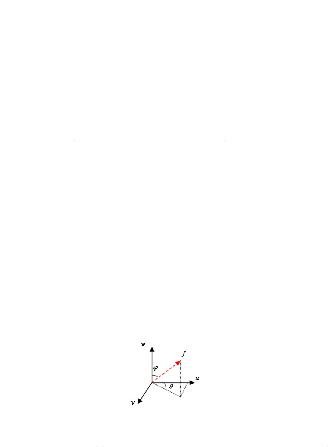
and h are the angles of the wave vector with w-axis and u–v plane in frequency domain ðu;
v
; wÞ (as
shown in Fig. 1), and
r
is the width of Gaussian envelop in ðx; y; bÞ domain. ðx
c
; y
c
; b
c
Þ indicates the position for signal
analysis.
Let V be a 3D hyperspectral image cube of an X Y region captured in B spectral bands. Vðx; y; bÞ is the signal information
of a sampled spatial location ðx; yÞ captured in spectral band b. The response of signal to wavelet
W
f ;h;
u
ðx; y; bÞ represents the
strength of variance with frequency amplitude f and orientation ð
u
; hÞ. The response of Vðx; y; bÞ to
W
f ;h;
u
ðx; y; bÞ is defined as:
H
f ;h;
u
ðx; y; bÞ¼ ðV W
f ;h;
u
Þðx; y; bÞ
ð2Þ
where denotes the convolution operation and jjcalculates the magnitude of the response.
H
f ;h;
u
ðx; y; bÞ reveals the infor-
mation of signal variances around location ðx; y; bÞ with center frequency f and orientation ðh;
u
Þ at joint spatial-spectrum
domains.
2.2. Pixel-level classification vs. image-level classification
This work studies 3D Gabor wavelet feature extraction for hyperspectral imagery classification on two levels, i.e., pixel-
level and image-level. In pixel-level classification such as material recognition in hyperspectral remote sensing data [37,45],
each pixel in a location ðx; y Þ across all B spectral bands, i.e.,Vðx; y; Þ, is treated as a learning target, and the task of classifi-
cation is to assign a class label for each pixel. In such case, after 3D Gabor wavelet transform, a pixel at Vðx; y; Þ yields a set of
responses f
H
f ;h;
u
ðx; y; 1Þ;
H
f ;h;
u
ðx; y; 2Þ; ...;
H
f ;h;
u
ðx; y; BÞg to a single 3D Gabor wavelet. By considering together all 3D Gabor
wavelets, each pixel sample therefore can be featured by a numeric vector that concatenates the pixel’s response sets to all
wavelets. A classifier needs to be trained to classify each pixel to different categories, e.g., road, grass and water, based on the
numeric feature vector.
In image-level classification like hyperspectral face recognition [14], each 3D hyperspectral cube is considered as a sam-
ple of a category and the target is to label a class for the whole image cube. In this case, each pixel on an image can serve as a
feature point for classifying the image. After transformed with a single 3D Gabor wavelet, a 3D hyperspectral cube Vð; ; Þ
of size X Y B can be represented by a response set containing the responses of all pixels across all bands to the wavelet,
i.e., f
H
f ;h;
u
ð1; 1; 1Þ;
H
f ;h;
u
ð1; 1; 2Þ; ...;
H
f ;h;
u
ðX; Y; BÞg. Accordingly, when transformed with all 3D Gabor wavelets, a 3D hyper-
spectral cube sample is represented as the concatenation of all response sets, each of which is subject to a unique wavelet.
Fig. 1. Three-dimensional frequency domain.
276 Z. Zhu et al. / Information Sciences 298 (2015) 274–287


