
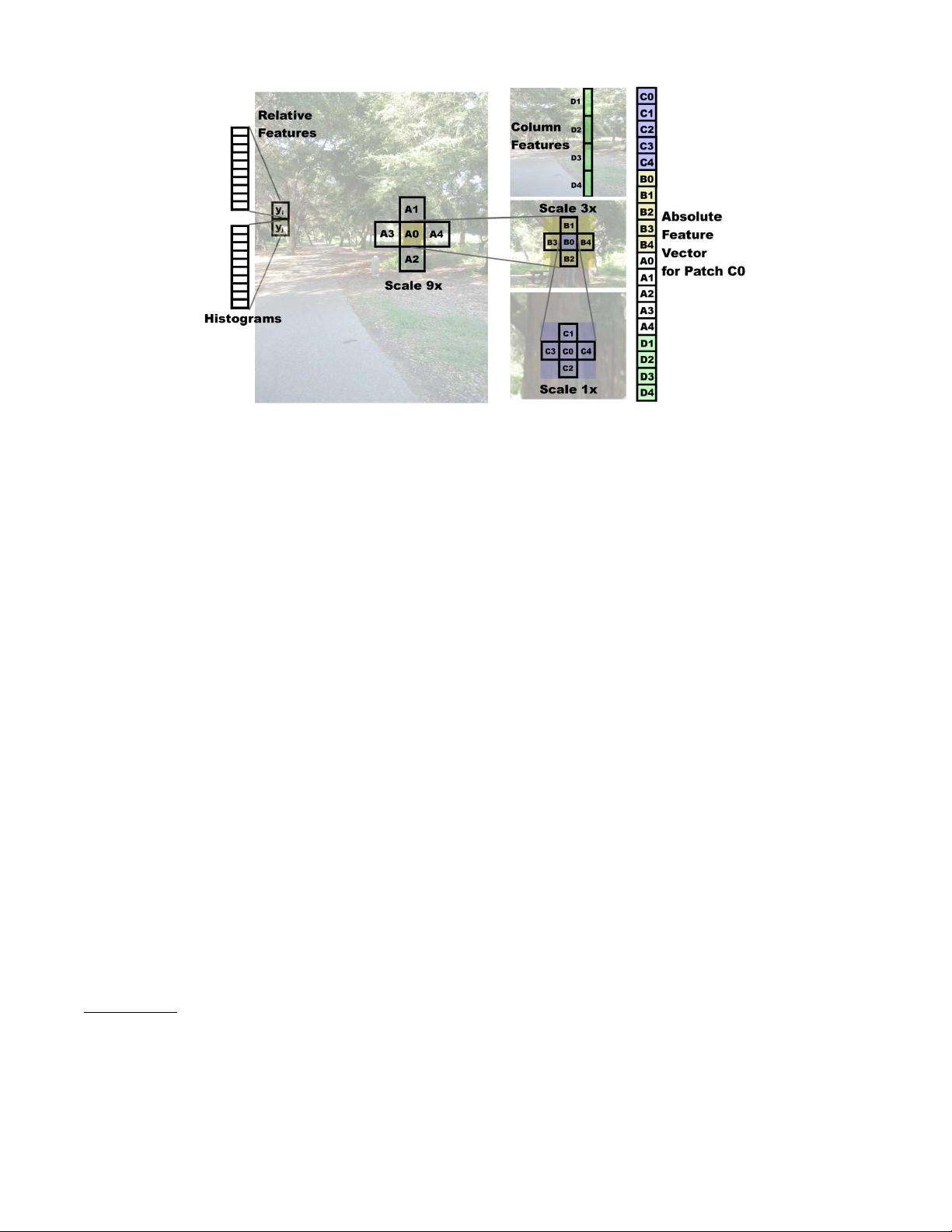
Figure 3: The absolute depth feature vector for a patch, which includes features from its immediate neighbors and
its more distant neighbors (at larger scales). The relative depth features for each patch use histograms of the filter
outputs.
absolute energy and sum squared energy respectively.
4
This gives us an initial feature vector of dimension 34.
To estimate the absolute depth at a patch, local im-
age features centered on the patch are insufficient, and
one has to use more global properties of the image. We
attempt to capture this information by using image fea-
tures extracted at multiple spatial scales (image resolu-
tions).
5
(See Fig. 3.) Objects at different depths exhibit
very different behaviors at different resolutions, and us-
ing multiscale features allows us to capture these vari-
ations
[
58
]
. For example, blue sky may appear similar
at different scales, but textured grass would not. In ad-
dition to capturing more global information, computing
features at multiple spatial scales also helps to account
for different relative sizes of objects. A closer object ap-
pears larger in the image, and hence will be captured
in the larger scale features. The same object when far
away will be small and hence be captured in the small
scale features. Features capturing the scale at which an
object appears may therefore give strong indicators of
depth.
To capture additional global features (e.g. occlusion
relationships), the features used to predict the depth of a
particular patch are computed from that patch as well as
the four neighboring patches. This is repeated at each of
the three scales, so that the feature vector at a patch in-
cludes features of its immediate neighbors, its neighbors
at a larger spatial scale (thus capturing image features
4
Our experiments using k ∈ {1, 2, 4} did not improve per-
formance noticeably.
5
The patches at each spatial scale are arranged in a grid
of equally sized non-overlapping regions that cover the entire
image. We use 3 scales in our experiments.
that are slightly further away in the image plane), and
again its neighbors at an even larger spatial scale; this
is illustrated in Fig. 3. Lastly, many structures (such as
trees and buildings) found in outdoor scenes show verti-
cal structure, in the sense that they are vertically con-
nected to themselves (things cannot hang in empty air).
Thus, we also add to the features of a patch additional
summary features of the column it lies in.
For each patch, after including features from itself and
its 4 neighbors at 3 scales, and summary features for its
4 column patches, our absolute depth feature vector x is
19 ∗ 34 = 646 dimensional.
4.2 Features for relative depth
We use a different feature vector to learn the dependen-
cies between two neighboring patches. Specifically, we
compute a 10-bin histogram of each of the 17 filter out-
puts |I ∗F
n
|, giving us a total of 170 features y
is
for each
patch i at scale s. These features are used to estimate
how the depths at two different locations are related. We
believe that learning these estimates requires less global
information than predicting absolute depth, but more
detail from the individual patches. For example, given
two adjacent patches of a distinctive, unique, color and
texture, we may be able to safely conclude that they
are part of the same object, and thus that their depths
are close, even without more global features. Hence, our
relative depth features y
ijs
for two neighboring patches
i and j at scale s will be the differences between their
histograms, i.e., y
ijs
= y
is
− y
js
.
5 Probabilistic Model
Since local images features are by themselves usually in-
sufficient for estimating depth, the model needs to reason
剩余15页未读,继续阅读

frankelly
- 粉丝: 1
- 资源: 13
 我的内容管理
展开
我的内容管理
展开


最新资源
- C++标准程序库:权威指南
- Java解惑:奇数判断误区与改进方法
- C++编程必读:20种设计模式详解与实战
- LM3S8962微控制器数据手册
- 51单片机C语言实战教程:从入门到精通
- Spring3.0权威指南:JavaEE6实战
- Win32多线程程序设计详解
- Lucene2.9.1开发全攻略:从环境配置到索引创建
- 内存虚拟硬盘技术:提升电脑速度的秘密武器
- Java操作数据库:保存与显示图片到数据库及页面
- ISO14001:2004环境管理体系要求详解
- ShopExV4.8二次开发详解
- 企业形象与产品推广一站式网站建设技术方案揭秘
- Shopex二次开发:触发器与控制器重定向技术详解
- FPGA开发实战指南:创新设计与进阶技巧
- ShopExV4.8二次开发入门:解决升级问题与功能扩展
资源上传下载、课程学习等过程中有任何疑问或建议,欢迎提出宝贵意见哦~我们会及时处理!
点击此处反馈


