


优化Ward BRDF评估与 Monte Carlo 算法详解
需积分: 9 94 浏览量
更新于2024-09-04
收藏 710KB PDF 举报
本篇文档主要讨论的是Ward BRDF(双向反射分布函数),这是一种在计算机图形学中广泛应用的非均匀BRDF模型,最初由Bruce Walter在1992年的论文中提出。相比于早期的BRDF模型,Ward BRDF具有显著的优势,包括参数简单易控、易于进行Monte Carlo采样且适用于模拟各向异性表面,以及能够较好地拟合实际测量的表面反射数据。
文档首先强调了Ward BRDF的实施细节可能不如其理论概念那么广泛为人所知,作者着重讲解如何有效地评估这种BRDF。评估方法可能涉及特定的数学公式和算法优化,以减少计算复杂度并提高效率,这对于实际应用中的性能至关重要。
接着,文档深入到Ward BRDF与Monte Carlo方法的结合。作者详细推导了与Ward BRDF相关的蒙特卡罗采样方案的概率密度函数,这是实现随机光照模拟和渲染的关键步骤。正确理解并使用这些权重有助于生成高质量的样本,进而提高渲染结果的逼真度和精度。
对于Ward BRDF的 isotropic版本(即各向同性情况),文档探讨了如何限制在特定方向空间区域内可能出现的最大BRDF值。这个界限对于理解和控制光照的散射效果是十分重要的,因为它可以帮助避免过度渲染或暗度过低的问题。
总结来说,这篇文档提供了对Ward BRDF的实用指导,涵盖了模型的高效评估、采样策略的理论基础以及如何处理不同类型的表面属性。对于任何从事计算机图形学特别是实时渲染领域的专业人士来说,理解和掌握这些细节无疑会提升他们的技术水平,并有助于创建更真实、高效的图像渲染系统。
Notes on the Ward BRDF
Bruce Walter
∗
Technical Report PCG-05-06
Cornell Program of Computer Graphics
April 29, 2005
Abstract
The anisotropic BRDF introduced in [Ward 1992] has become
widely used in computer graphics, but some important implemen-
tation details are less widely known. We discuss how to efficiently
evaluate the Ward BRDF. Then we derive the probability density
function for its associated Monte Carlo sampling scheme and the
correct weights to use with the generated samples. Finally for the
isotropic version, we describe how to bound the maximum possible
BRDF value over a region of (direction) space.
1 Introduction
The Ward BRDF (Bidirectional Reflectance Distribution Function)
was introduced in [Ward 1992] as an empirical model to fit mea-
sured BRDF (i.e. surface reflectance) data. It has several advan-
tages over the prior BRDF models and has become widely used in
the computer graphics community. It uses only a few simple pa-
rameters making it easy to control, can be sampled efficiently for
Monte Carlo, can model anisotropic surfaces, and was shown to fit
reasonably well to measured BRDF data.
The purpose of this paper is to clarify and correct some important
implementation details of the Ward BRDF. We discuss how to effi-
ciently evaluate the BRDF in Section 2. Monte Carlo BRDF sam-
pling is required for many rendering algorithms, and hence, Ward
provided an efficient sampling scheme with his BRDF. However he
did not provide the associated probability density function, which
for mathematical accuracy, is needed to correctly weight the gen-
erated samples. We both discuss how to derive such probability
density functions in general in Section 3, and present the specific
results for the Ward BRDF in Equation 10.
Another powerful, though less widely used, BRDF operation is
the ability to bound its maximum value over a range of directions.
In Section 4, we discuss how to cheaply cheaply and tightly bound
the isotropic Ward BRDF over a set of directions defined by a spa-
tial bounding volume.
1.1 Notation
We will be working extensively with directions in 3D, which
we will denote in boldface (e.g., v). In actual use, these di-
rections are typically represented as normalized 3D vectors (e.g.,
v = [v
x
, v
y
, v
z
], where v
2
x
+v
2
y
+v
2
z
= 1). Directions can also be rep-
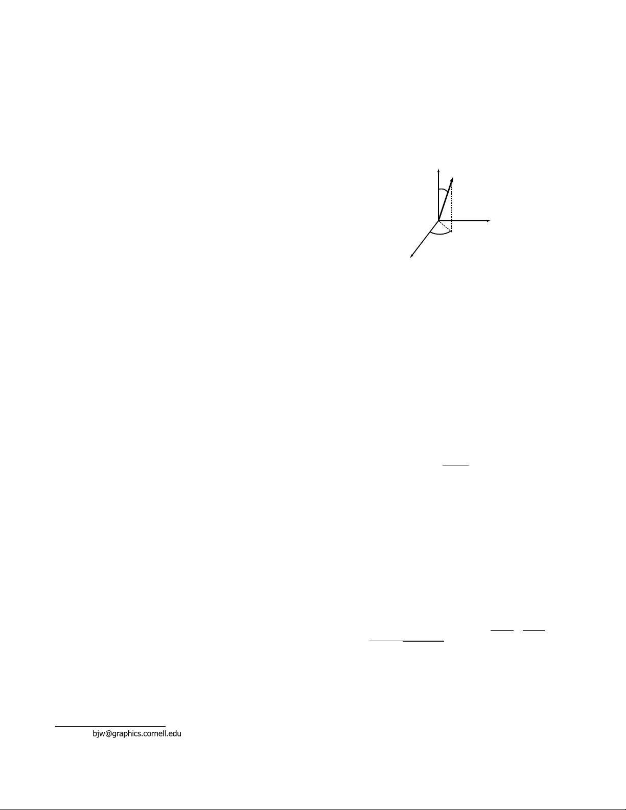
resented as two angles, θ and φ , using spherical polar coordinates
as illustrated in Figure 1. We will usually subscript these angles
with the direction that they are describing. We can convert between
the spherical angles and the 3D unit vector representations using:
(θ, φ ) ⇔
sinθ cos φ, sin θ sin φ , cos θ
(1)
The scalar dot product of two directions is equal to the cosine
of the angle between them (e.g., v ·z = cos θ
v
). When using 3D
vectors, the dot product can be computed by summing the products
of the corresponding components (e.g., u ·v = u
x
v
x
+ u
y
v
y
+ u
z
v
z
).
∗
email:
x
y
z
v
θ
v
φ
v
Figure 1: Spherical polar coordinates example. The direction v
can be fully described by two angles θ
v
and φ
v
. θ
v
is the angle
between v and the z-axis. φ
v
is the angle between the x-axis and v’s
projection onto the x-y plane.
A BRDF (Bidirectional Reflectance Distribution Function) de-
scribes how light is scattered at a surface. At a surface point it is a
function of two directions (an incident direction i and an outgoing
direction o) and written as f
r
(i,o). It is often convenient to con-
struct a coordinate frame on the surface where the z-axis is the same
of the local surface normal, n, and the x and y axes lie in the tangent
plane of the surface as shown in Figure 2. For anisotropic BRDFs,
the x and y axes must match the principle directions of anisotropy,
while they can be chosen arbitrarily for isotropic BRDFs.
The Ward BRDF uses the half direction h that is defined to be
halfway between the incident and out directions. It can be com-
puted by adding i and o as 3D vectors and then renormalizing:
h =
i + o
ki + ok
(2)
The half angle is motivated by microfacet BRDFs and produces
more realistic highlights than alternatives such as Phong (e.g., see
[Fisher 1994; Ngan et al. 2004]).
2 Ward BRDF
The original Ward BRDF is defined as the sum of two components
[Ward 1992, Equation 5a]. The first is a diffuse term, ρ
d
/π. Dif-
fuse components are relatively simple and already well understood,
so we will ignore the diffuse component for the remainder of this
paper. The second component is a gaussian anisotropic gloss lobe
defined by three parameters, ρ
s
, α
x
, and α
y
, as:
f
r
(i,o) =
ρ
s
4πα
x
α
y
√
cosθ
i
cosθ
o
e
−tan
2
θ
h
cos
2
φ
h
α
2
x
+
sin
2
φ
h
α
2
y
(3)
where ρ
s
controls the magnitude of the lobe, and α
x
and α
y
control
the width of the lobe in the two principal directions of anisotropy.
If α
x
= α
y
then the lobe is isotropic (i.e. invariant under surface
rotations around the surface normal).
Just after defining his BRDF, Ward presents an approximation
that is intended to be computationally cheaper [Ward 1992, Equa-
tion 5b]. There is no reason to ever use this approximation. The fol-
lowing vector equation is both exact and cheaper to compute than
下载后可阅读完整内容,剩余4页未读,立即下载
2134 浏览量
2025-04-17 上传
126 浏览量
125 浏览量
101 浏览量
2025-04-17 上传
2025-04-17 上传
2025-04-17 上传
2025-04-17 上传
2025-04-17 上传

softant2008
- 粉丝: 4
 我的内容管理
展开
我的内容管理
展开


最新资源
- 掌握这11个Spring核心jar包,助你快速搭建项目
- 经典XP系统图标资源下载指南
- 免安装迷你PDF阅读器:快速且低内存占用
- 深入解析Hugflash元素提取技术
- HarmonyOS2下的音乐文件夹管理器Harmony使用指南
- SAP HANA NGDBC驱动使用与安装详解
- JACOB库文件下载指南:jacob.jar与jacob.dll
- 软件加密解密技术的内幕解析
- JSP实现的玉米生长动态模拟系统研究
- 深入解析J1939协议在C语言中的实现方法
- 深入解析:IE缓存提取工具IEContent的使用
- 掌握allpairs测试工具:有效组合条件自动化测试
- 模拟高速公路交通的面向代理编程项目
- CSDN创刊号:《C&C++杂志》电子版首发珍藏
- 电脑版二维码生成器:快速创建二维码文件
- 采购现金预算表:高效管理采购成本的参考工具