多相机密集RGB-D SLAM系统研究
需积分: 5 172 浏览量
更新于2024-08-26
收藏 3.14MB PDF 举报
"Dense RGB-D SLAM with Multiple Cameras[1].pdf"
本文主要探讨了使用多个RGB-D(红绿蓝深度)相机进行稠密SLAM(Simultaneous Localization and Mapping,即同时定位与建图)的系统,该系统具有加速场景重建和提高定位精度的潜力。通过使用多个安装的传感器和扩大有效视场,可以显著提升SLAM系统的性能。文章重点研究了两个关键问题:一是如何在传感器视野小或不重叠的情况下进行系统标定,以最大限度地增加有效视场;二是如何有效地融合来自不同传感器的位置信息。
首先,对于多相机系统的标定,由于各相机的视野可能只有小部分重合或完全不重合,这给传统的单目或双目相机标定方法带来了挑战。作者提出了一种新的标定方法,旨在优化各个相机的参数,使得整个系统能够覆盖更大的空间范围,从而扩大了SLAM的可工作区域。这种方法可能包括对每个相机的内外参进行独立标定,然后通过共享的特征点来调整它们之间的相对位置关系,以实现多相机间的精确同步和配准。
其次,多相机SLAM系统中的数据融合是另一个关键技术。不同的RGB-D传感器可能提供不同的视点和深度信息,因此需要一种有效的融合策略来确保全局一致性和精度。文中可能涉及了滤波器方法(如扩展卡尔曼滤波器EKF或无迹卡尔曼滤波器UKF)、优化方法(如图优化)或者其他高级的数据融合技术,用于整合来自多个源的定位信息,降低不确定性并减少漂移。
此外,论文可能还讨论了实时处理和计算效率的问题,这对于实际应用至关重要。多相机设置会增加数据量,因此需要高效的算法来处理大量输入,并保持系统运行的实时性。这可能涉及到并行计算、分布式处理或者特定硬件加速的利用。
"Dense RGB-D SLAM with Multiple Cameras[1].pdf"这篇论文详细研究了多相机环境下的稠密SLAM技术,包括系统标定和数据融合策略,这些研究成果对于增强现实、机器人导航、3D建模等领域有着重要的实践意义。通过解决这些问题,可以构建更强大、更稳健的多传感器SLAM系统,以应对复杂环境下的高精度定位和三维重建需求。
Sensors 2018, 18, 2118 3 of 12
2.
We extend the state-of-the-art ElasticFusion [
20
] to a multi-camera system to get a better dense
RGB-D SLAM.
Sensors 2018, 18, x 3 of 11
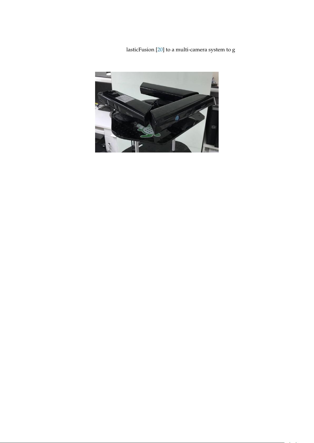
Figure 1. Example of three-Kinect arrangement.
2. Extrinsic Calibration of Multiple Cameras
2.1. Odometer-Based Extrinsic Calibration
We run RGB-D visual odometry (VO) for each camera in a feature-rich scene to estimate a set of
camera poses which is required for the subsequent step of hand–eye calibration. Our RGB-D VO
method is similar to [21], which is the classical VO method for RGB-D SLAM. We perform a dense
iterated close point (ICP) method to estimate the camera pose, using a projective data association
algorithm [22] to obtain correspondence and a point-to-plane error metric for pose optimization.
Then we solve the optimization problem based on the GPU’s parallelized processing pipeline. The
point-to-plane error energy for the desired camera pose estimate T is
E=
(
()−
()
)
∙
.
∈
(1)
We track the current camera frame by aligning a live surface measurement (
,
) against the
model prediction from the previous frame (
,
), where Ω⊂ℕ
is the image space domain, v
is vertex, n is normal, and k is the timestamp. With the VO method, we obtain a set of camera poses.
Then we use the hand–eye calibration method of [7] to estimate each camera-odometry
transformation. The unknown camera-odometry transformation is estimated in two steps. In the first
step, the rotation cost function is minimized to estimate the pitch and roll angles of the camera-
odometry transformation. In the second step, the translation cost function is minimized to estimate
the yaw angle and the camera-odometry translation. The relationship between camera and robot can
be expressed as a rotation formula and a translation formula as
=
,
(2)
−
=
(
)
−
.
(3)
In the above, the rotation is represented by quaternion, and the translation by a vector. The
robot’s transformation between time i and time i + 1 is denoted by the vector
and the unit
quaternion
, which can be obtained from the robot’s inertial measurement unit.
and
represent the camera’s transformation between time i and time i + 1 which can be obtained by the
above VO method.
and
represent the transformation between the robot and the camera. In
the first step, we decompose the unknown unit quaternion
into three unit quaternions,
corresponding to Z–X–Y. Euler angles α, β, γ as
=
(
)
(
,
)
.
(4)
Since both
and
() represent rotations around the z axis, they satisfy commutative law.
After simplifying Function (2), the rotation residual term becomes
Figure 1. Example of three-Kinect arrangement.
2. Extrinsic Calibration of Multiple Cameras
2.1. Odometer-Based Extrinsic Calibration
We run RGB-D visual odometry (VO) for each camera in a feature-rich scene to estimate a set
of camera poses which is required for the subsequent step of hand–eye calibration. Our RGB-D
VO method is similar to [
21
], which is the classical VO method for RGB-D SLAM. We perform
a dense iterated close point (ICP) method to estimate the camera pose, using a projective data
association algorithm [
22
] to obtain correspondence and a point-to-plane error metric for pose
optimization. Then we solve the optimization problem based on the GPU’s parallelized processing
pipeline. The point-to-plane error energy for the desired camera pose estimate T is
E =
∑
u∈Ω
((
Tv
k
(
u
)
− v
k−1
(
u
))
·n
k−1
)
2
. (1)
We track the current camera frame by aligning a live surface measurement (
v
k
,
n
k
) against the
model prediction from the previous frame (
v
k−1
,
n
k−1
), where
Ω ⊂ N
2
is the image space domain,
v
is
vertex, n is normal, and k is the timestamp. With the VO method, we obtain a set of camera poses.
Then we use the hand–eye calibration method of [
7
] to estimate each camera-odometry
transformation. The unknown camera-odometry transformation is estimated in two steps. In the
first step, the rotation cost function is minimized to estimate the pitch and roll angles of the
camera-odometry transformation. In the second step, the translation cost function is minimized
to estimate the yaw angle and the camera-odometry translation. The relationship between camera and
robot can be expressed as a rotation formula and a translation formula as
R
i+1
R
i
q
R
C
q =
R
C
q
C
i+1
C
i
q, (2)
R
R
i+1
R
i
q
− I
R
C
p = R
R
C
q
C
i+1
C
i
p −
R
i+1
R
i
p. (3)
In the above, the rotation is represented by quaternion, and the translation by a vector. The robot’s
transformation between time i and time i + 1 is denoted by the vector
R
i+1
R
i
p
and the unit quaternion
R
i+1
R
i
q
, which can be obtained from the robot’s inertial measurement unit.
C
i+1
C
i
p
and
C
i+1
C
i
q
represent
the camera’s transformation between time i and time i + 1 which can be obtained by the above VO
method.
R
C
p
and
R
C
q
represent the transformation between the robot and the camera. In the first step,
剩余11页未读,继续阅读
2019-04-01 上传
2024-01-11 上传
2024-09-02 上传
2022-07-15 上传
2022-07-15 上传
2021-03-23 上传
2022-07-15 上传
2022-09-22 上传
2023-12-20 上传


donghanruchen
- 粉丝: 0
- 资源: 37
 我的内容管理
展开
我的内容管理
展开


最新资源
- Aspose资源包:转PDF无水印学习工具
- Go语言控制台输入输出操作教程
- 红外遥控报警器原理及应用详解下载
- 控制卷筒纸侧面位置的先进装置技术解析
- 易语言加解密例程源码详解与实践
- SpringMVC客户管理系统:Hibernate与Bootstrap集成实践
- 深入理解JavaScript Set与WeakSet的使用
- 深入解析接收存储及发送装置的广播技术方法
- zyString模块1.0源码公开-易语言编程利器
- Android记分板UI设计:SimpleScoreboard的简洁与高效
- 量子网格列设置存储组件:开源解决方案
- 全面技术源码合集:CcVita Php Check v1.1
- 中军创易语言抢购软件:付款功能解析
- Python手动实现图像滤波教程
- MATLAB源代码实现基于DFT的量子传输分析
- 开源程序Hukoch.exe:简化食谱管理与导入功能
