REED
et
al.:
LMS
ADAPTIVE FILTER-STATIC BEHAVIOR
563
-
+
M-POINT
-
c
din)
-
FFT
t
-
:
0
M-POINT
IFFT
COMPLEX
1-TAP
LMS
AF
II
w
LMS AF
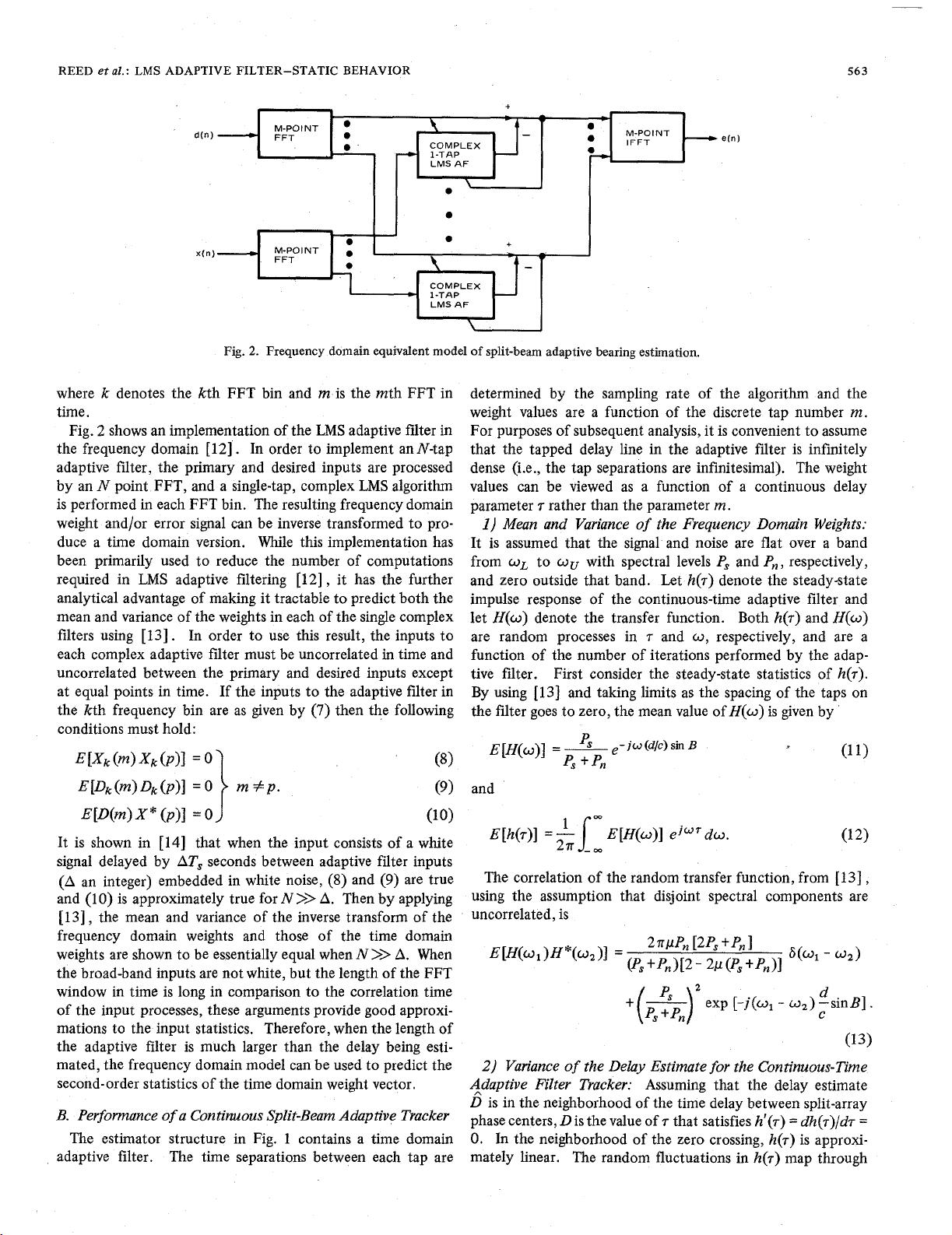
Fig.
2.
Frequency domain equivalent model
of
split-beam adaptive bearing estimation.
where
k
denotes the kth FFT bin and
m
is the mth FFT in
time.
Fig.
2
shows an implementation of the
LMS
adaptive filter
in
the frequency domain
[
121
.
In order to implement an N-tap
adaptive filter, the primary and desired inputs are processed
by an
N
point FFT, and a single-tap, complex
LMS
algorithm
is performed in each FFT bin. The resulting frequency domain
weight and/or error signal can be inverse transformed to pro-
duce a time domain version. While this implementation has
been primarily used to reduce the number of computations
required in
LMS
adaptive filtering
[12]
,
it has the further
analytical advantage of making
it
tractable to predict both the
mean and variance of the weights in each of the single complex
filters using
[
131
.
In order to use this result, the inputs to
each complex adaptive filter must be uncorrelated in time and
uncorrelated between the primary and desired inputs except
at equal points in time. If the inputs to the adaptive filter in
the kth frequency bin are as given by
(7)
then the following
conditions must hold:
E
[xk
(m>
xk
(PI]
=
EIDk(m)Dk(P)l
=o
m
fp.
(9)
i
(8)
E[Nm)X*
(P)l
=
0
(10)
It is shown in
[
141
that when the input consists of a white
signal delayed by
AT,
seconds between adaptive filter inputs
(A
an integer) embedded in white noise,
(8)
and
(9)
are true
and
(10)
is approximately true for
N
>>
A.
Then by applying
[
131
,
the mean and variance
of
the inverse transform of the
frequency domain weights and those of the time domain
weights are shown to be essentially equal when
N
>>
A.
When
the broad-band inputs are not white, but the length of the FFT
window in time is long in comparison to the correlation time
of the input processes, these arguments provide good approxi-
mations to the input statistics. Therefore, when the length of
the adaptive filter is much larger than the delay being esti-
mated, the frequency domain model can be used to predict the
second-order statistics of the time domain weight vector.
B. Performance
of
a
Continuous Split-Beam Adaptive Tracker
The estimator structure in Fig.
1
contains a time domain
adaptive filter. The time separations between each tap are
determined by the sampling rate of the algorithm and the
weight values are a function of the discrete tap number
m.
For purposes of subsequent analysis, it is convenient to assume
that the tapped delay line in the adaptive filter is infinitely
dense (i.e., the tap separations are infinitesimal). The weight
values can be viewed as a function of a continuous delay
parameter
7
rather than the parameter
m.
1)
Mean and Variance of the Frequency Domain Weights:
It is assumed that the signal and noise are flat over
a
band
from
oL
to
ou
with spectral levels
P,
and
P,,
respectively,
and zero outside that band. Let
h(7)
denote the steady-state
impulse response of the continuous-time adaptive filter and
let
H(o)
denote the transfer function. Both
h(7)
and
H(o)
are random processes in
7
and
o,
respectively, and are a
function
of
the number of iterations performed by the adap-
tive filter. First consider the steady-state statistics of
h(7).
By using
[13]
and taking limits as the spacing of the taps
on
the filter goes to zero, the mean value
of
H(o)
is given by
and
loo
E[h(7)]
=
E[H(o)] eiwrdo.
(12)
The correlation of the random transfer function, from
[13]
,
using the assumption that disjoint spectral components are
uncorrelated, is
(13)
2)
Variance of the Delay Estimate for the Continuous-Time
4daptive Filter Tracker:
Assuming that the delay estimate
D
is in the neighborhood of the time delay between split-array
phase centers,
D
is the value of
7
that satisfies
h'(7)
=
dh(.r)/d.r
=
0.
In the neighborhood
of
the zero crossing,
h(7)
is approxi-
mately linear. The random fluctuations in
h(7)
map through


