7740 IEEE TRANSACTIONS ON GEOSCIENCE AND REMOTE SENSING, VOL. 52, NO. 12, DECEMBER 2014
B. JSRM
In HSI, neighboring pixels that belong to the same material
usually are strongly correlated with each other. In [30], the
JSRM is introduced to capture such spatial correlations by
assuming that neighboring pixels within a region of fixed size
can be jointly represented by a few common atoms from a
structural dictionary. Specifically, the size of a region centered
at test pixel y
1
is denoted by W × W , and pixels within such
a region are denoted by {y
i
}
i=1,...,W ×W
. These pixels can also
be stacked into a matrix Y =[y
1
, y
2
,...,y
W ×W
], of the size
M × (W × W ). The matrix can be compactly represented as
Y =[y
1
, y
2
,...,y
W ×W
]=[Dα
1
, Dα
2
,...,Dα
W ×W
]
= D[α
1
, α
2
,...,α
W ×W
]=DA (8)
where A =[α
1
, α
2
,...,α
W ×W
] is the sparse coefficients
matrix corresponding to Y. Since the positions of nonzero
coefficients in [α
1
, α
2
,...,α
W ×W
] determine the indexes
of the selected atoms in D, the JSRM enables neighboring
pixels[y
1
, y
2
,...,y
W ×W
] to be represented by a small set of
common atoms, by enforcing a few nonzero rows on the sparse
coefficients matrix A. Then, matrix A can be obtained by
solving the following optimization problem:
ˆ
A =argmin
A
Y − DA
F
subject to A
row,0
≤ K (9)
where A
row,0
denotes the joint sparse norm, which is used
to select a number of the most representative nonzero rows in
A, and ·
F
is the Frobenius norm. A variant of the OMP
algorithm called the simultaneous OMP (SOMP) [34] can be
used to efficiently obtain an approximate solution. Note that,
enforcing the structured constraints (e.g., mixed L
1,2
[33] and
manifold [45]) on (9) may lead to a better sparse coefficients
matrix, but also create a higher computational cost. After
ˆ
A
is recovered, the label of test pixel y
1
can be decided by the
minimal total error, i.e.,
ˆc =argmin
c
Y − D
c
ˆ
A
c
F
,c=1,...,C (10)
where
ˆ
A
c
denotes the rows in
ˆ
A associated with the cth class.
By incorporating spatial information of local regions, the
JSRM can deliver much better classification results, in terms
of accuracy, compared to the pixelwise SRC model. However,
the region size (or, as we call it, the region scale) greatly affects
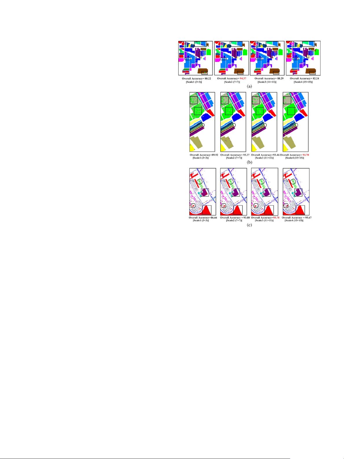
the classification performance. Fig. 1 shows the classification
results for the JSRM with varied region scales for three different
data sets. As can be observed in Fig. 1, different regions
favor different region scales. Specifically, detailed or near-edge
regions require a comparatively small region scale (e.g., ellipse
regions in Fig. 1) whereas large region scales are preferred for
smooth areas (e.g., rectangle regions in Fig. 1). Therefore, it is
not trivial to determine an optimal region scale for the JSRM.
III. P
ROPOSED MASR FOR HSI CLASSIFICATION
A. Multiscale Spatial Information in HSI
Given one test pixel y
1
in HSI, its T neighboring regions
are selected of different scales (sizes). Pixels within the se-
Fig. 1. Influence of region scales on the JSRM algorithm (Overall Accuracy
values are given in percentage). (a) Classification results obtained by the JSRM
algorithm on the Indian Pine image with region scales varying from 3 × 3to
15 × 15. (b) Classification results obtained by the JSRM algorithm on the Sali-
nas image with region scales varying from 3 × 3to15× 15. (c) Classification
results obtained by the JSRM algorithm on the University of Pavia image with
region scales varying from 3 × 3to15× 15.
lected regions can be arranged to construct the corresponding
multiscale matrix Y
multiscale
=[Y
1
,...,Y
t
,...,Y
T
], where
Y
t
includes pixels from the tth scale region. In HSI, regions
of different scales usually exhibit distinct spatial structures
and characteristics. Nonetheless, since all the different scales
correspond to the same test pixel y
1
, they should provide com-
plementary yet correlated information, which can be utilized to
classify y
1
more accurately.
B. Multiscale Spatial Information in HSI
Suppose that we have one structural dictionary D and the
multiscale matrix [Y
1
,...,Y
t
,...,Y
T
] for the test pixel y
1
.
Then, all the sparse representation problems of T scales (9) can
be rewritten together as
{
ˆ
A
t
}
T
t=1
=argmin
{A
t
}
T
t=1
Y
t
− DA
t
F
subject to A
t
row,0
≤ K ∀ 1 ≤ t ≤ T (11)
where [A
1
,...,A
t
,...,A
T
] are the sparse coefficients for
[Y
1
,...,Y
t
,...,Y
T
], which can constitute a multiscale
sparse coefficients matrix A
multiscale
. Such a problem can be
solved by separately applying the SOMP algorithm [34] on


