没有合适的资源?快使用搜索试试~ 我知道了~
首页分布式系统入门:保罗·西维洛蒂的讲解
分布式系统入门:保罗·西维洛蒂的讲解
需积分: 9 3 下载量 63 浏览量
更新于2024-07-23
收藏 741KB PDF 举报
"《分布式系统入门:保罗·西维洛蒂博士》是一本由保罗·西维洛蒂博士编著的计算机科学与工程领域的教材,发表于2007年的春季学期,隶属于美国俄亥俄州立大学。该书深入浅出地介绍了分布式系统的基本概念和技术,主要围绕布尔逻辑、谓词演算和量化等核心主题展开。 第1章首先探讨了布尔逻辑、谓词和量词的概念。作者通过函数、布尔值和谓词来构建基础理论框架。'到处括号'(Everywhere Brackets)的概念被用来表达系统的全局性质,而谓词演算则讨论了等价性、析取、合取、蕴含和否定等基本逻辑运算。此外,作者还引入了不一致性的概念(Discrepance),强调了在分布式系统中逻辑一致性的重要性。 章节2转向了计算模型的介绍,包括引用文献的列表。在这个部分,程序的概念被明确定义,区分了简单的赋值操作、多重赋值、带有条件的行动(Guarded Actions)以及程序的顺序执行。作者通过实例,如FindMax算法,展示如何用这些概念来理解和设计分布式系统的执行流程。读者可以学习到如何通过操作直观地理解程序的行为以及何时会终止。 视觉化编程的方法也被提及,通过有向图或状态转换图帮助读者更好地理解分布式系统中的控制流和状态变化。这种可视化工具有助于解释分布式环境中的复杂交互和同步问题。 总体而言,《分布式系统入门》为学习者提供了一个坚实的理论基础,使他们能够掌握分布式系统的设计原则、逻辑结构以及执行机制,这对于理解现代互联网、云计算和分布式计算技术至关重要。无论是对初学者还是研究者来说,这本书都是理解和实践分布式系统不可或缺的参考资料。"
资源详情
资源推荐
4 CHAPTER 1. BOOLEANS, PREDICATES, AND QUANTIFICATION
and obvious. Nevertheless, this distinction quickly b ecomes blurred when we
consider operations. The familiar operations on booleans (e.g., ∧ , ∨ ) can
also be applied to predicates! They are technically different operations, since
they have different signatures, but confusion can arise because the same symbol
is usually used.
∧ : boolean × boolean → boolean
∧ : predicate × predicate →
Typically, the operator being used is clear from context (i.e., from the types
of the arguments). We could add subscripts to distinguish these operators, but
this would needlessly clutter our expressions and mask many of the common-
alities between these different versions of fundamentally similar functions (with
fundamentally similar properties).
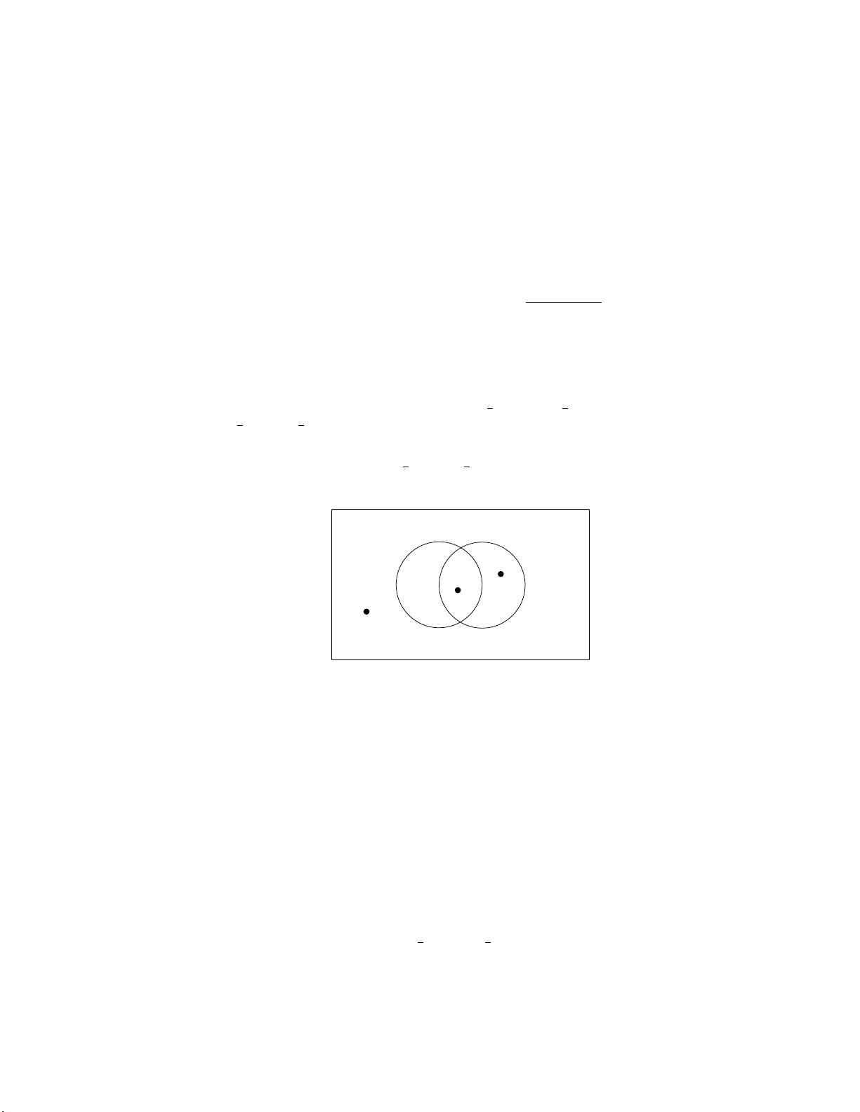
For example, consider the predicates is tall and is heavy . The expression
is tall ∧ is heavy denotes a predicate! It is therefore a function that can be
applied to particular elements of its domain, for example:
(is tall ∧ is heavy).Jeff
This results in a boolean. See Figure 1.2 for a graphical representation.
S
is_tallis_heavy
Sindhu
Jeff
Mikko
Figure 1.2: The Conjunction of Two Predicates
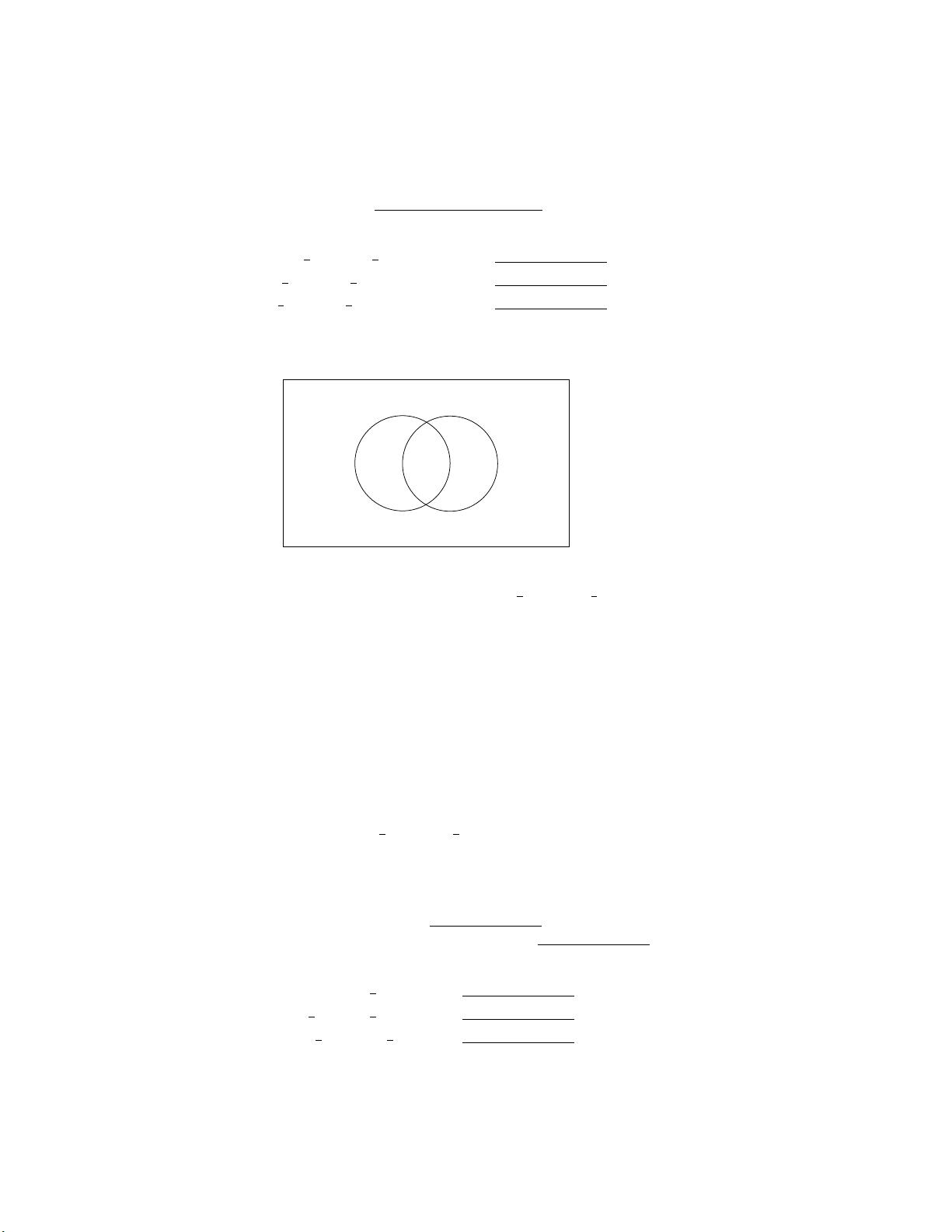
In this way, a simple operator on boolean ( ∧ ) has been elevated to operate
on functions that map to boolean. This overloading of a single symbol is called
lifting. Of course, the process of lifting can continue, elevating the operator to
apply to functions that map to functions that map to boolean. And so on.
Lifting can be applied to the constants true and false as well. These symbols
have been introduced as the elements of the set of boolean. But they can also be
lifted to be predicates (the former mapping to true everywhere, and the latter
to false). This leads us into the topic of what is meant by “everywhere”...
1.2.4 Everywhere Brackets
Consider the following expression:
is tall ≡ is heavy
1.2. PRELIMINARIES 5
Notice that this expression is a . Thus, we can evaluate
it at various points in its domain, for example:
(is tall ≡ is heavy).Joe is
(is tall ≡ is heavy).Mikko is
(is tall ≡ is heavy).Sindhu is
In this way, you can complete Figure 1.3 by shading the areas in which the
element is mapped to true.
S
is_tallis_heavy
Figure 1.3: Graphical Representation of is tall ≡ is heavy
But what if we wanted to talk about the equivalence of the two predicates
themselves? In other words, what if we want to state the claim “Being tall is
the same as being heavy”? This claim is either true or false. It is not true
sometimes and false other times. So what is going on here?
The problem is that the claim really involves an implicit quantification.
Claiming that “Being tall is the same as being heavy” can more precisely be
restated as “For every person, being tall is the same as being heavy”. Thus,
we could use explicit quantification to state our claim. This issue turns out
to be so pervasive, however, that it is worth introducing a short-hand for this
quantification. We write:
[is tall ≡ is heavy]
The domain over which the quantification occurs is understood from context.
When it matters, it is almost always the state space of some program under
consideration. The square brackets are known as “everywhere brackets”.
Notice that the expression is now a . Indeed we can enclose
any predicate with everywhere brackets, resulting in a .
[is heavy] is
[is tall ∨ is heavy] is
[is tall ∨ ¬is tall] is
6 CHAPTER 1. BOOLEANS, PREDICATES, AND QUANTIFICATION
1.3 The Predicate Calculus
1.3.1 Equivalence
We begin the introduction of the predicate calculus with arguably its most fun-
damental operator: equivalence. This operator is written ≡ and pronounced
“equivals”. Intuitively, X ≡ Y means that both are true or both are false.
Why not use the more common operator = (pronounced “equals”)? The
main reason for choosing a different symbol is that the equals operator has a
sp ecial meaning when there are multiple occurrences on the same line. For
example, one might see:
sqrt.16 = 4 = 2
2
This is called “chaining” and it is really a short-hand for writing two conjuncts:
(sqrt.16 = 4) ∧ (4 = 2
2
)
Equivals can also appear multiple times on the same line, but—in general—
we do not intend this to represent chaining. An expression with multiple occur-
rences of equivals is evaluated (or simplified) directly. For example:
false ≡ true
| {z }
≡ false
≡ false
| {z }
But, rewriting this expression as if chaining were the intended interpretation
leads to a different result:
(false ≡ true)
| {z }
∧ (true ≡ false)
| {z }
∧
| {z }
Formally, equivalence is defined by its axioms.
Axiom 1. Associativity of ≡ .
[((X ≡ Y ) ≡ Z) ≡ (X ≡ (Y ≡ Z))]
This means that in an expression with multiple ≡ ’s, it doesn’t matter
how it is parenthesized. Therefore, the parentheses will be omitted, and we are
free to evaluate the equivalences in any order we wish. For example, we might
write [X ≡ Y ≡ Z] , and we would then be free to interpret this as either
[(X ≡ Y ) ≡ Z] or as [X ≡ (Y ≡ Z)] .
1.3. THE PREDICATE CALCULUS 7
Axiom 2. Commutativity of ≡ .
[X ≡ Y ≡ Y ≡ X]
Here we make use of the associativity of ≡ to write the axiom without
parentheses. The resulting axiom is quite rich. It captures the property of
commutativity, with:
[(X ≡ Y ) ≡ (Y ≡ X)]
It also, however, can be parenthesized as follows:
[X ≡ (Y ≡ Y ) ≡ X]
This exposes an interesting fact: the expression (Y ≡ Y ) is both the left and
right identity of ≡ . An identity element is worth naming, and we do so next.
Axiom 3. Definition of true.
[Y ≡ Y ≡ true]
Again, notice the effect of different placements of parentheses. By interpret-
ing this axiom as [Y ≡ (Y ≡ true)] we see that true is indeed the (right)
identity of ≡ . In other words, there is no difference between writing [Y ] and
[Y ≡ true] .
1.3.2 Disjunction
While ≡ is interesting, just one operator is a little limiting. So, we introduce
a new operator, called disjunction and written ∨ (pronounced“or”). To reduce
the number of parentheses, we define an order of operations: ∨ is defined to
bind more tightly than ≡ .
We define this new operator by the following four axioms.
Axiom 4. Associativity of ∨ .
[X ∨ (Y ∨ Z) ≡ (X ∨ Y ) ∨ Z]
Axiom 5. Commutativity of ∨ .
[X ∨ Y ≡ Y ∨ X]
Axiom 6. Idempotence of ∨ .
[X ∨ X ≡ X]
The last axiom describes how our two operators interact with each other.
Axiom 7. Distribution of ∨ over ≡ .
[X ∨ (Y ≡ Z) ≡ (X ∨ Y ) ≡ (X ∨ Z)]
The definition of these two operators (i.e., the axioms given above) form the
foundation of our presentation of the predicate calculus. There are many other
choices for where to begin this presentation. A different set of axioms could
have been chosen and then the associativity of ∨ , for example, derived as a
theorem.
8 CHAPTER 1. BOOLEANS, PREDICATES, AND QUANTIFICATION
1.3.3 Proof Format
The axioms above give the basic properties of our operators. They can be used
to derive further properties of these operators as theorems. A theorem must be
proven from a set of axioms and theorems that have already been proven. To
carry out these proofs, we will use a precise notation. This notation will help us
structure our proofs so they are easy to read and verify. Perhaps surprisingly,
this format also frequently makes proofs easier to write since it will often suggest
the next step to be carried out.
Proofs are carried out in a calculational style. Each step in the proof involves
the application of one (or more) axioms or theorems. Each step is annotated
with a hint for the reader justifying that step. Each step should be small enough
that a reader can be easily convinced the step is correct. Beware of steps that
involve the application of multiple axioms or theorems! These steps are often
where trouble arises. As you write proofs, you will develop a feel for the appro-
priate granularity of these steps: Too small and the proof is pedantic and hard
to follow, but too large and the pro of is obscure and hard to follow. Some ax-
ioms are used so ubiquitously they are frequently omitted (e.g., commutativity
of ≡ and of ∨ ). As a rule of thumb, error on the side of thoroughness.
As an general example of our calculational pro of notation, consider a proof
of [A ≡ B] . One such proof might take the form:
A
≡ { reason why [A ≡ C] }
C
≡ { reason why [C ≡ B] }
B
2
A (less nice) alternative for such a proof would be:
A ≡ B
≡ { reason why [A ≡ B ≡ D] }
D
≡ { reason why [D ≡ true] }
true
2
Writing proofs in this way will give us a common structure in which to read
each other’s proofs. It will also encourage a nice discipline of justifying steps in a
precise manner. Notice, also, that expressions written in this format have a very
different meaning than their straight-line counterparts. That is, the meaning of
A
≡
C
≡
B
剩余153页未读,继续阅读
williamshyy
- 粉丝: 0
- 资源: 1
上传资源 快速赚钱
- 我的内容管理 展开
- 我的资源 快来上传第一个资源
- 我的收益 登录查看自己的收益
- 我的积分 登录查看自己的积分
- 我的C币 登录后查看C币余额
- 我的收藏
- 我的下载
- 下载帮助
最新资源
- OptiX传输试题与SDH基础知识
- C++Builder函数详解与应用
- Linux shell (bash) 文件与字符串比较运算符详解
- Adam Gawne-Cain解读英文版WKT格式与常见投影标准
- dos命令详解:基础操作与网络测试必备
- Windows 蓝屏代码解析与处理指南
- PSoC CY8C24533在电动自行车控制器设计中的应用
- PHP整合FCKeditor网页编辑器教程
- Java Swing计算器源码示例:初学者入门教程
- Eclipse平台上的可视化开发:使用VEP与SWT
- 软件工程CASE工具实践指南
- AIX LVM详解:网络存储架构与管理
- 递归算法解析:文件系统、XML与树图
- 使用Struts2与MySQL构建Web登录验证教程
- PHP5 CLI模式:用PHP编写Shell脚本教程
- MyBatis与Spring完美整合:1.0.0-RC3详解
资源上传下载、课程学习等过程中有任何疑问或建议,欢迎提出宝贵意见哦~我们会及时处理!
点击此处反馈
安全验证
文档复制为VIP权益,开通VIP直接复制
信息提交成功