Since there are many inverse operators in Appendix 1, it requires
to study the invertibility of these matrices. The analysis is shown in
Appendix 2.
To verify the approximate linear relationship between ||x
∗
1
||
1
and
ɛ, many test pairs of A and y are generated. After performing these
tests, it is found that the approximate linear relationship between
||x
∗
1
||
1
and ɛ is valid for all these pairs of A and y. Only three
types of experiments are presented below to support the proposed
assertions because of the page limit.
2.1 Experiment 1: Signals satisfying the condition in (3)
Here, the relationship between ||x
∗
1
||
1
and ɛ when the condition in (3)
is satisfied is investigated. In this experiment, m = 40 and n = 100.
All the elements of A are independently drawn from a zero mean
Gaussian distribution. Then,
A
i
for i =1,…,100 is further
normalised to a unit energy vector. There are five non-zero
elements in α
0
and the locations of these elements are selected
randomly with their polarities also being chosen randomly. The
amplitude of the smallest non-zero element of α
0
is set to 0.2 and
the amplitudes of other elements are set to 1. Using this α
0
, y is
obtained. Obviously, x
∗
0
=
a
0
. x
∗
0
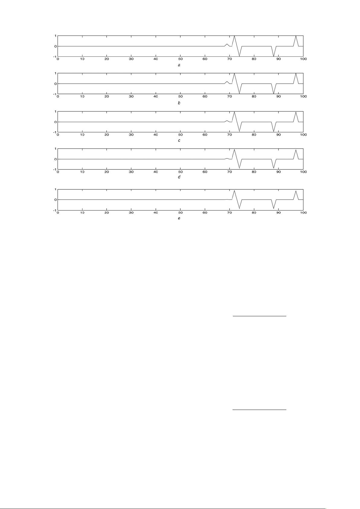
is shown in Fig. 1a.When ɛ =0,
||y||
2
/20, ||y||
2
/10 and 3||y||
2
/20, the corresponding x
∗
1
are shown
in Figs. 1b–e, respectively. It is shown in [7] that x
∗
0
= x
∗
1
when
ρ ≤ (1/5). This can also be verified from Figs. 1a–b. Although a
large value of ɛ allows a large bound on ||Ax
∗
1
− y||
2
, it results to a
small value of ||x
∗
1
||
1
. In other words, we have a high scarcity of
x
∗
1
. It can be seen in Fig. 1e that the total number of the non-zero
elements in x
∗
1
is 4 when ɛ = 3||y||
2
/20. This further demonstrates
the reason for the relaxation on the L
2
norm specification.
To further investigate the relationship between ||x
∗
1
||
1
and ɛ, 100
test pairs of A and y are generated as described in the above. For
each test pair of A and y, various values of ɛ, denoted as ɛ
i
, are
obtained via uniformly sampling in the range [0,||y||
2
]. Denote the
corresponding solution of (4) as x
∗
1
i
for i =1, 2, …, N. It is found
that an approximate linear relationship exists between ||x
∗
1
i
||
1
and
ɛ
i
for all these 100 test pairs of A and y. For an illustration
purpose, (1
i
, ||x
∗
1
i
||
1
) of one of the test pairs of A and y are shown
in Fig. 2. A straight line linear regression fitof(1
i
, ||x
∗
1
i
||
1
)
denoted as f (ɛ
i
)=k*ɛ
i
+ b* is also shown in Fig. 2. The relative L
2
norm error is defined as
N
i=1
|f (1
i
) −||x
∗
1
i
||
1
|
2
N
i=1
(||x
∗
1
i
||
1
)
2
. (5)
It is found that the L
2
norm error is around 2.3%. On the other hand,
it is also found that an approximate linear relationship exists between
x
∗
1
i
− x
∗
0
2
( x
∗
1
i
− x
∗
0
2
is the root mean squares error between x
∗
1
i
and x
∗
0
) and ɛ
i
for all these 100 test pairs of A and y. For an
illustration purpose, (1
i
, x
∗
1
i
− x
∗
0
2
) of one of the test pairs of A
and y are shown in Fig. 3. A linear regression fitof
(1
i
, x
∗
1
i
− x
∗
0
2
) denoted as g(1
i
) =
k
∗
1
i
+
b
∗
is also shown in
Fig. 3. The relative L
2
norm error is defined as
N
i=1
|g(1
i
) −||x
∗
1
i
||
1
|
2
N
i=1
(||x
∗
1
i
||
1
)
2
. (6)
It is found that the relative L
2
norm error is around 1.8%. All these
100 test pairs of A and y show similar results.
2.2 Experiment 2: Trials using randomly generated data
Since condition in (3) is difficult to satisfy in many practical
situations, x
∗
0
= x
∗
1
only happens in ideal scenarios. It is therefore
Fig. 1 Amplitude of the smallest non-zero element of α
0
is set to 0.2 and the amplitudes of other elements are set to 1
ax
∗
0
b–ex
∗
1
for ɛ =0,||y||
2
/20, ||y||
2
/10 and 3||y||
2
/20, respectively
IET Signal Process., 2015, Vol. 9, Iss. 9, pp. 670–680
672
&
The Institution of Engineering and Technology 2015


