深度学习驱动的单图像超分辨率：CVPR方法与创新

下载需积分: 46 | PDF格式 | 2.07MB | 更新于2024-09-11 | 129 浏览量 | 举报

"CVPR图像超分辨率"是计算机视觉领域的一个重要研究方向，主要关注如何利用深度学习技术提升图像的细节质量和清晰度，尤其是在单张图像的高分辨率重建上。该论文由Chao Dong、Chen Change Loy、Kaiming He和Xiaoou Tang等研究人员提出，他们提出了一种深度卷积神经网络（Deep Convolutional Neural Network，DCNN）方法来处理这一问题。在传统图像超分辨率（Single Image Super-Resolution，SISR）方法中，通常依赖于稀疏编码或者基于分解的技术，这些方法可能需要对图像的不同特征进行逐个处理。然而，这篇论文提出的方法则完全不同，它通过构建一个端到端的深度学习模型，将低分辨率图像作为输入，直接学习并生成高分辨率的输出。这种方法的优势在于能够联合优化所有层，从而提高整体性能。论文的核心贡献在于设计了一种轻量级的深度卷积网络结构，这种网络在保持高恢复质量的同时，实现了较快的实时处理速度，适合于实际应用中的在线使用。作者通过探索不同的网络结构和参数设置，成功地实现了性能与速度之间的平衡，使得方法既能在复杂场景下保持良好的效果，又能在实时性方面满足需求。此外，该研究还扩展了他们的网络架构，使其能够同时处理三通道的彩色图像，这进一步增强了图像的复原质量，尤其是在处理颜色丰富的场景时，显示出更好的整体重建能力。因此，该工作不仅推动了图像超分辨率技术的发展，也为实际图像处理应用提供了一个有效且高效的解决方案。 "CVPR图像超分辨率"这一研究展示了深度学习在图像处理领域的强大潜力，通过创新的网络设计和优化策略，它在提高图像质量的同时，兼顾了计算效率，对于提升图像处理技术的整体水平具有重要意义。

of them has analyzed the SR performance of different chan-

nels, and the necessity of recovering all three channels.

2.2 Convolutional Neural Networks (CNN)

Convolutional neural networks date back decades [26] and

deep CNNs have recently shown an explosive popularity

partially due to its success in image classiﬁcation [18], [25].

They have also been successfully applied to other computer

vision ﬁelds, such as object detection [33], [50], face recogni-

tion [38], and pedestrian detection [34]. Several factors are

of central importance in this progress: (i) the efﬁcient train-

ing implementation on modern powerful GPUs [25], (ii) the

proposal of the rectiﬁed linear unit (ReLU) [32] which

makes convergence much faster while still presents good

quality [25], and (iii) the easy access to an abundance of

data (like ImageNet [9]) for training larger models. Our

method also beneﬁts from these progresses.

2.3 Deep Learning for Image Restoration

There have been a few studies of using deep learning tech-

niques for image restoration. The multi-layer perceptron

(MLP), whose all layers are fully-connected (in contrast to

convolutional), is applied for natural image denoising [3]

and post-deblurring denoising [35]. More closely related to

our work, the convolutional neural network is applied for

natural image denoising [21] and removing noisy patterns

(dirt/rain) [12]. These restoration problems are more or less

denoising-driven. Cui et al. [5] propose to embed auto-

encoder networks in their super-resolution pipeline under

the notion internal example-based approach [16]. The deep

model is not speciﬁcally designed to be an end-to-end solu-

tion, since each layer of the cascade requires independent

optimization of the self-similarity search process and the

auto-encoder. On the contrary, the proposed SRCNN opti-

mizes an end-to-end mapping. Further, the SRCNN is faster

at speed. It is not only a quantitatively superior method, but

also a practically useful one.

3CONVOLUTIONAL NEURAL NETWORKS FOR

SUPER-RESOLUTION

3.1 Formulation

Consider a single low-resolution image, we ﬁrst upscale it to

the desired size using bicubic interpolation, which is the

only pre-processing we perform.

Let us denote the interpo-

lated image as Y. Our goal is to recover from Y an image

F ðYÞ that is as similar as possible to the ground truth high-

resolution image X. For the ease of presentation, we still call

Y a “low-resolution” image, although it has the same size as

X. We wish to learn a mapping F, which conceptually con-

sists of three operations:

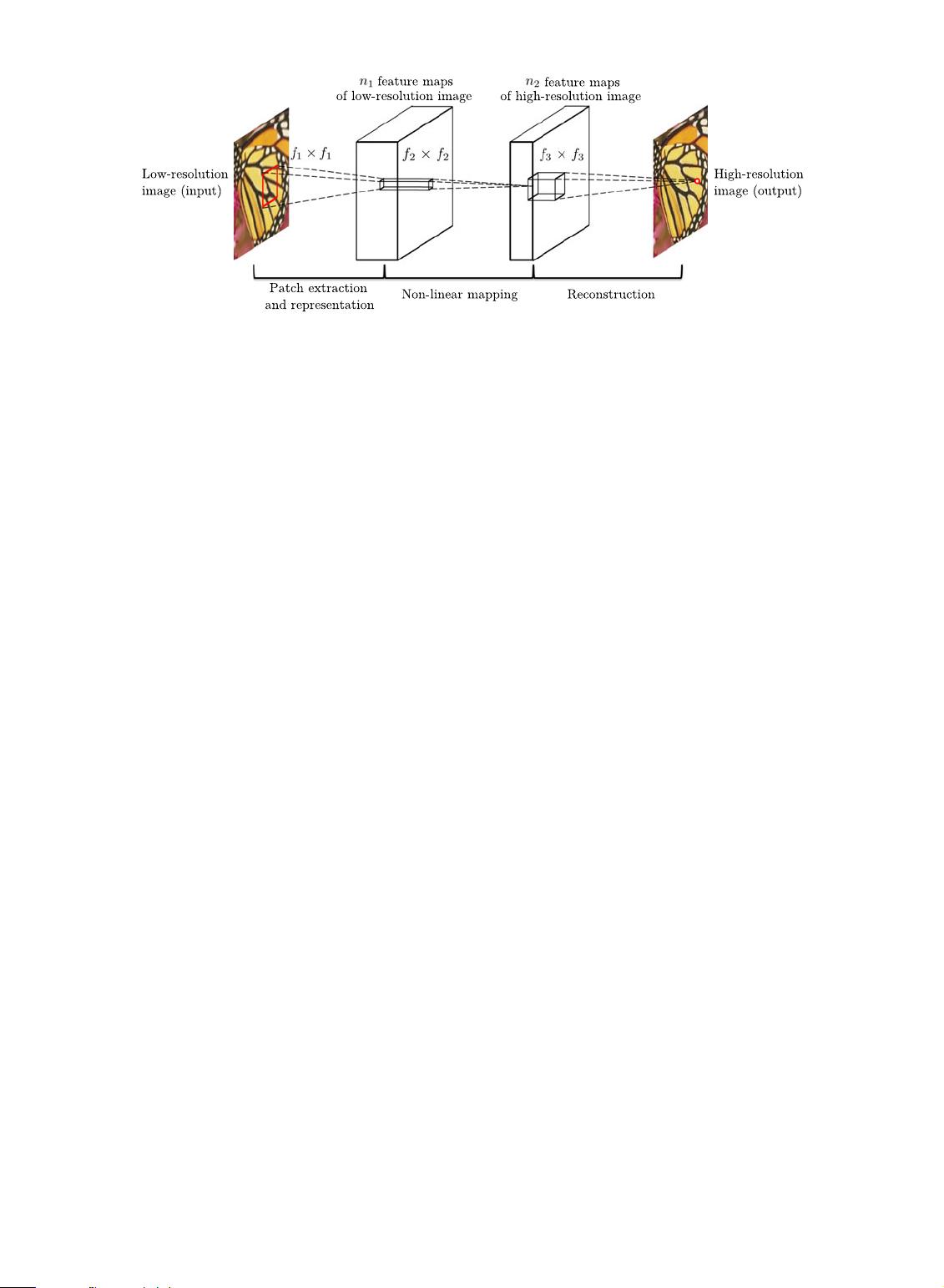
1) Patch extraction and representation. this operation

extracts (overlapping) patches from the low-resolu-

tion image Y and represents each patch as a high-

dimensional vector. These vectors comprise a set of

feature maps, of which the number equals to the

dimensionality of the vectors.

2) Non-linear mapping. this operation nonlinearly maps

each high-dimensional vector onto another high-

dimensional vector. Each mapped vector is concep-

tually the representation of a high-resolution patch.

These vectors comprise another set of feature maps.

3) Reconstruction. this operation aggregates the above

high-resolution patch-wise representations to gener-

ate the ﬁnal high-resolution image. This image is

expected to be similar to the ground truth X.

We will show th at all these operations form a convolu-

tional neural network. An overview of the network is

depicted in Fig. 2. Next we detail our deﬁnition of each

operation.

3.1.1 Patch Extraction and Representation

A popular strategy in image restoration (e.g., [1]) is to

densely extract patches and then represent them by a set of

pre-trained bases such as PCA, DCT, Haar, etc. This is

equivalent to convolving the image by a set of ﬁlters, each

of which is a basis. In our formulation, we involve the opti-

mization of these bases into the optimization of the network.

Formally, our ﬁrst layer is expressed as an operation F

ðYÞ¼max 0;W

 Y þ B

ðÞ; (1)

Fig. 2. Given a low-resolution image Y, the ﬁrst convolutional layer of the SRCNN extracts a set of feature maps. The second layer maps these

feature maps nonlinearly to high-resolution patch representations. The last layer combines the predictions within a spatial neighbourhood to produce

the ﬁnal high-resolution image F ðYÞ.

3. Bicubic interpolation is also a convolutional operation, so it can be

formulated as a convolutional layer. However, the output size of this

layer is larger than the input size, so there is a fractional stride. To take

advantage of the popular well-optimized implementations such as

cuda-convnet [25], we exclude this “layer” from learning.

DONG ET AL.: IMAGE SUPER-RESOLUTION USING DEEP CONVOLUTIONAL NETWORKS 297

剩余12页未读，继续阅读

qq_33691974

粉丝: 1
资源: 3

深度学习驱动的单图像超分辨率：CVPR方法与创新

NTIRE2019_EDRN:我对NTIRE2019真正超分辨率的解决方案

图像超分辨率重建（ 适合初学超分辨率重建使用 图像超分辨率 SR工具箱）

基于深度学习的图像超分辨率（paper集）

CVPR 2023 超分辨率

cvpr视频超分辨率

超分辨率重建matlab代码-HBPN:CVPR2019中用于图像超分辨率的分层反投影网络（HBPN）

CVPR2013基于字典学习的图像超分辨率代码

PyTorch实施残差密集网络以实现图像超分辨率 CVPR 2018

SMSR:[CVPR 2021]探索图像超分辨率中的稀疏性以进行有效推理

2017CVPR 超分辨率大赛总结文档

最新资源

图像超分辨率重建（适合初学超分辨率重建使用图像超分辨率 SR工具箱）